Note
This page was generated from
peakvi_in_R.ipynb.
Interactive online version:
![]() .
Some tutorial content may look better in light mode.
.
Some tutorial content may look better in light mode.
ATAC-seq analysis in R#
In this tutorial, we go over how to use scvi-tools functionality in R for analyzing ATAC-seq data. We will closely follow the PBMC tutorial from Signac, using scvi-tools when appropriate. In particular, we will
Use PeakVI for dimensionality reduction and differential accessiblity for the ATAC-seq data
Use scVI to integrate the unpaired ATAC-seq dataset with a match scRNA-seq dataset of PBMCs
This tutorial requires Reticulate. Please check out our installation guide for instructions on installing Reticulate and scvi-tools.
Loading and processing data with Signac#
[1]:
system("wget https://cf.10xgenomics.com/samples/cell-atac/1.0.1/atac_v1_pbmc_10k/atac_v1_pbmc_10k_filtered_peak_bc_matrix.h5")
system("wget https://cf.10xgenomics.com/samples/cell-atac/1.0.1/atac_v1_pbmc_10k/atac_v1_pbmc_10k_singlecell.csv")
system("wget https://cf.10xgenomics.com/samples/cell-atac/1.0.1/atac_v1_pbmc_10k/atac_v1_pbmc_10k_fragments.tsv.gz")
system("wget https://cf.10xgenomics.com/samples/cell-atac/1.0.1/atac_v1_pbmc_10k/atac_v1_pbmc_10k_fragments.tsv.gz.tbi")
[1]:
library(Signac)
library(Seurat)
library(GenomeInfoDb)
library(EnsDb.Hsapiens.v75)
library(ggplot2)
library(patchwork)
set.seed(1234)
Attaching SeuratObject

Loading required package: BiocGenerics


Attaching package: ‘BiocGenerics’


The following objects are masked from ‘package:stats’:

    IQR, mad, sd, var, xtabs


The following objects are masked from ‘package:base’:

    anyDuplicated, append, as.data.frame, basename, cbind, colnames,
    dirname, do.call, duplicated, eval, evalq, Filter, Find, get, grep,
    grepl, intersect, is.unsorted, lapply, Map, mapply, match, mget,
    order, paste, pmax, pmax.int, pmin, pmin.int, Position, rank,
    rbind, Reduce, rownames, sapply, setdiff, sort, table, tapply,
    union, unique, unsplit, which.max, which.min


Loading required package: S4Vectors

Loading required package: stats4


Attaching package: ‘S4Vectors’


The following objects are masked from ‘package:base’:

    expand.grid, I, unname


Loading required package: IRanges

Loading required package: ensembldb

Loading required package: GenomicRanges

Loading required package: GenomicFeatures

Loading required package: AnnotationDbi

Loading required package: Biobase

Welcome to Bioconductor

    Vignettes contain introductory material; view with
    'browseVignettes()'. To cite Bioconductor, see
    'citation("Biobase")', and for packages 'citation("pkgname")'.


Loading required package: AnnotationFilter


Attaching package: 'ensembldb'


The following object is masked from 'package:stats':

    filter
Pre-processing#
We follow the original tutorial to create the Seurat object with ATAC data.
[2]:
counts <- Read10X_h5(filename = "atac_v1_pbmc_10k_filtered_peak_bc_matrix.h5")
metadata <- read.csv(
  file = "atac_v1_pbmc_10k_singlecell.csv",
  header = TRUE,
  row.names = 1
)

chrom_assay <- CreateChromatinAssay(
  counts = counts,
  sep = c(":", "-"),
  genome = 'hg19',
  fragments = 'atac_v1_pbmc_10k_fragments.tsv.gz',
  min.cells = 10,
  min.features = 200
)

pbmc <- CreateSeuratObject(
  counts = chrom_assay,
  assay = "peaks",
  meta.data = metadata
)
Warning message in sparseMatrix(i = indices[] + 1, p = indptr[], x = as.numeric(x = counts[]), :
"'giveCsparse' has been deprecated; setting 'repr = "T"' for you"
Computing hash

Warning message in CreateSeuratObject.Assay(counts = chrom_assay, assay = "peaks", :
"Some cells in meta.data not present in provided counts matrix."
[3]:
pbmc
An object of class Seurat
87561 features across 8728 samples within 1 assay
Active assay: peaks (87561 features, 0 variable features)
[4]:
pbmc[['peaks']]
ChromatinAssay data with 87561 features for 8728 cells
Variable features: 0
Genome: hg19
Annotation present: FALSE
Motifs present: FALSE
Fragment files: 1
We add gene annotation information to facilitate downstream functionality.
[5]:
# extract gene annotations from EnsDb
annotations <- GetGRangesFromEnsDb(ensdb = EnsDb.Hsapiens.v75)

# change to UCSC style since the data was mapped to hg19
seqlevelsStyle(annotations) <- 'UCSC'
genome(annotations) <- "hg19"

# add the gene information to the object
Annotation(pbmc) <- annotations
Fetching data...
OK

Parsing exons...
OK
Defining introns...
OK
Defining UTRs...
OK
Defining CDS...
OK

aggregating...

Done

Fetching data...
OK

Parsing exons...
OK
Defining introns...
OK
Defining UTRs...
OK
Defining CDS...
OK

aggregating...

Done

Fetching data...
OK

Parsing exons...
OK
Defining introns...
OK
Defining UTRs...
OK
Defining CDS...
OK

aggregating...

Done

Fetching data...
OK

Parsing exons...
OK
Defining introns...
OK
Defining UTRs...
OK
Defining CDS...
OK

aggregating...

Done

Fetching data...
OK

Parsing exons...
OK
Defining introns...
OK
Defining UTRs...
OK
Defining CDS...
OK

aggregating...

Done

Fetching data...
OK

Parsing exons...
OK
Defining introns...
OK
Defining UTRs...
OK
Defining CDS...
OK

aggregating...

Done

Fetching data...
OK

Parsing exons...
OK
Defining introns...
OK
Defining UTRs...
OK
Defining CDS...
OK

aggregating...

Done

Fetching data...
OK

Parsing exons...
OK
Defining introns...
OK
Defining UTRs...
OK
Defining CDS...
OK

aggregating...

Done

Fetching data...
OK

Parsing exons...
OK
Defining introns...
OK
Defining UTRs...
OK
Defining CDS...
OK

aggregating...

Done

Fetching data...
OK

Parsing exons...
OK
Defining introns...
OK
Defining UTRs...
OK
Defining CDS...
OK

aggregating...

Done

Fetching data...
OK

Parsing exons...
OK
Defining introns...
OK
Defining UTRs...
OK
Defining CDS...
OK

aggregating...

Done

Fetching data...
OK

Parsing exons...
OK
Defining introns...
OK
Defining UTRs...
OK
Defining CDS...
OK

aggregating...

Done

Fetching data...
OK

Parsing exons...
OK
Defining introns...
OK
Defining UTRs...
OK
Defining CDS...
OK

aggregating...

Done

Fetching data...
OK

Parsing exons...
OK
Defining introns...
OK
Defining UTRs...
OK
Defining CDS...
OK

aggregating...

Done

Fetching data...
OK

Parsing exons...
OK
Defining introns...
OK
Defining UTRs...
OK
Defining CDS...
OK

aggregating...

Done

Fetching data...
OK

Parsing exons...
OK
Defining introns...
OK
Defining UTRs...
OK
Defining CDS...
OK

aggregating...

Done

Fetching data...
OK

Parsing exons...
OK
Defining introns...
OK
Defining UTRs...
OK
Defining CDS...
OK

aggregating...

Done

Fetching data...
OK

Parsing exons...
OK
Defining introns...
OK
Defining UTRs...
OK
Defining CDS...
OK

aggregating...

Done

Fetching data...
OK

Parsing exons...
OK
Defining introns...
OK
Defining UTRs...
OK
Defining CDS...
OK

aggregating...

Done

Fetching data...
OK

Parsing exons...
OK
Defining introns...
OK
Defining UTRs...
OK
Defining CDS...
OK

aggregating...

Done

Fetching data...
OK

Parsing exons...
OK
Defining introns...
OK
Defining UTRs...
OK
Defining CDS...
OK

aggregating...

Done

Fetching data...
OK

Parsing exons...
OK
Defining introns...
OK
Defining UTRs...
OK
Defining CDS...
OK

aggregating...

Done

Fetching data...
OK

Parsing exons...
OK
Defining introns...
OK
Defining UTRs...
OK
Defining CDS...
OK

aggregating...

Done

Fetching data...
OK

Parsing exons...
OK
Defining introns...
OK
Defining UTRs...
OK
Defining CDS...
OK

aggregating...

Done

Fetching data...
OK

Parsing exons...
OK
Defining introns...
OK
Defining UTRs...
OK
Defining CDS...
OK

aggregating...

Done

Warning message in .Seqinfo.mergexy(x, y):
"The 2 combined objects have no sequence levels in common. (Use
  suppressWarnings() to suppress this warning.)"
Warning message in .Seqinfo.mergexy(x, y):
"The 2 combined objects have no sequence levels in common. (Use
  suppressWarnings() to suppress this warning.)"
Warning message in .Seqinfo.mergexy(x, y):
"The 2 combined objects have no sequence levels in common. (Use
  suppressWarnings() to suppress this warning.)"
Warning message in .Seqinfo.mergexy(x, y):
"The 2 combined objects have no sequence levels in common. (Use
  suppressWarnings() to suppress this warning.)"
Warning message in .Seqinfo.mergexy(x, y):
"The 2 combined objects have no sequence levels in common. (Use
  suppressWarnings() to suppress this warning.)"
Warning message in .Seqinfo.mergexy(x, y):
"The 2 combined objects have no sequence levels in common. (Use
  suppressWarnings() to suppress this warning.)"
Warning message in .Seqinfo.mergexy(x, y):
"The 2 combined objects have no sequence levels in common. (Use
  suppressWarnings() to suppress this warning.)"
Warning message in .Seqinfo.mergexy(x, y):
"The 2 combined objects have no sequence levels in common. (Use
  suppressWarnings() to suppress this warning.)"
Warning message in .Seqinfo.mergexy(x, y):
"The 2 combined objects have no sequence levels in common. (Use
  suppressWarnings() to suppress this warning.)"
Warning message in .Seqinfo.mergexy(x, y):
"The 2 combined objects have no sequence levels in common. (Use
  suppressWarnings() to suppress this warning.)"
Warning message in .Seqinfo.mergexy(x, y):
"The 2 combined objects have no sequence levels in common. (Use
  suppressWarnings() to suppress this warning.)"
Warning message in .Seqinfo.mergexy(x, y):
"The 2 combined objects have no sequence levels in common. (Use
  suppressWarnings() to suppress this warning.)"
Warning message in .Seqinfo.mergexy(x, y):
"The 2 combined objects have no sequence levels in common. (Use
  suppressWarnings() to suppress this warning.)"
Warning message in .Seqinfo.mergexy(x, y):
"The 2 combined objects have no sequence levels in common. (Use
  suppressWarnings() to suppress this warning.)"
Warning message in .Seqinfo.mergexy(x, y):
"The 2 combined objects have no sequence levels in common. (Use
  suppressWarnings() to suppress this warning.)"
Warning message in .Seqinfo.mergexy(x, y):
"The 2 combined objects have no sequence levels in common. (Use
  suppressWarnings() to suppress this warning.)"
Warning message in .Seqinfo.mergexy(x, y):
"The 2 combined objects have no sequence levels in common. (Use
  suppressWarnings() to suppress this warning.)"
Warning message in .Seqinfo.mergexy(x, y):
"The 2 combined objects have no sequence levels in common. (Use
  suppressWarnings() to suppress this warning.)"
Warning message in .Seqinfo.mergexy(x, y):
"The 2 combined objects have no sequence levels in common. (Use
  suppressWarnings() to suppress this warning.)"
Warning message in .Seqinfo.mergexy(x, y):
"The 2 combined objects have no sequence levels in common. (Use
  suppressWarnings() to suppress this warning.)"
Warning message in .Seqinfo.mergexy(x, y):
"The 2 combined objects have no sequence levels in common. (Use
  suppressWarnings() to suppress this warning.)"
Warning message in .Seqinfo.mergexy(x, y):
"The 2 combined objects have no sequence levels in common. (Use
  suppressWarnings() to suppress this warning.)"
Warning message in .Seqinfo.mergexy(x, y):
"The 2 combined objects have no sequence levels in common. (Use
  suppressWarnings() to suppress this warning.)"
Warning message in .Seqinfo.mergexy(x, y):
"The 2 combined objects have no sequence levels in common. (Use
  suppressWarnings() to suppress this warning.)"
Computing QC metrics#
We compute the same QC metrics as the original tutorial. We leave it to the reader to follow the excellent Signac tutorial for understanding what these quantities represent.
[6]:
# compute nucleosome signal score per cell
pbmc <- NucleosomeSignal(object = pbmc)

# compute TSS enrichment score per cell
pbmc <- TSSEnrichment(object = pbmc, fast = FALSE)

# add blacklist ratio and fraction of reads in peaks
pbmc$pct_reads_in_peaks <- pbmc$peak_region_fragments / pbmc$passed_filters * 100
pbmc$blacklist_ratio <- pbmc$blacklist_region_fragments / pbmc$peak_region_fragments
Extracting TSS positions

Finding + strand cut sites

Finding - strand cut sites

Computing mean insertion frequency in flanking regions

Normalizing TSS score
[7]:
options(repr.plot.width=14, repr.plot.height=4)
VlnPlot(
  object = pbmc,
  features = c('pct_reads_in_peaks', 'peak_region_fragments',
               'TSS.enrichment', 'blacklist_ratio', 'nucleosome_signal'),
  pt.size = 0.1,
  ncol = 5
)
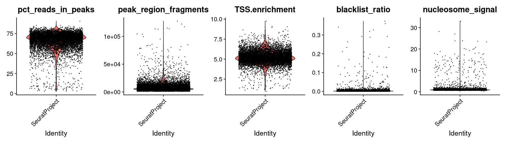
[8]:
pbmc <- subset(
  x = pbmc,
  subset = peak_region_fragments > 3000 &
    peak_region_fragments < 20000 &
    pct_reads_in_peaks > 15 &
    blacklist_ratio < 0.05 &
    nucleosome_signal < 4 &
    TSS.enrichment > 2
)
pbmc
An object of class Seurat
87561 features across 7060 samples within 1 assay
Active assay: peaks (87561 features, 0 variable features)
Dimensionality reduction (PeakVI)#
Creating an AnnData object#
We follow the standard workflow for converting between Seurat and AnnData.
[9]:
library(reticulate)
library(sceasy)
use_python("/home/adam/.pyenv/versions/3.9.7/bin/python", required = TRUE)
sc <- import("scanpy", convert = FALSE)
scvi <- import("scvi", convert = FALSE)
[10]:
adata <- convertFormat(pbmc, from="seurat", to="anndata", main_layer="counts", assay="peaks", drop_single_values=FALSE)
print(adata) # Note generally in Python, dataset conventions are obs x var
AnnData object with n_obs × n_vars = 7060 × 87561
    obs: 'orig.ident', 'nCount_peaks', 'nFeature_peaks', 'total', 'duplicate', 'chimeric', 'unmapped', 'lowmapq', 'mitochondrial', 'passed_filters', 'cell_id', 'is__cell_barcode', 'TSS_fragments', 'DNase_sensitive_region_fragments', 'enhancer_region_fragments', 'promoter_region_fragments', 'on_target_fragments', 'blacklist_region_fragments', 'peak_region_fragments', 'nucleosome_signal', 'nucleosome_percentile', 'TSS.enrichment', 'TSS.percentile', 'pct_reads_in_peaks', 'blacklist_ratio'
    var: 'count', 'percentile'
Run the standard PeakVI workflow#
[11]:
scvi$model$PEAKVI$setup_anndata(adata)
None
[12]:
pvi <- scvi$model$PEAKVI(adata)
pvi$train()
None
[13]:
# get the latent represenation
latent = pvi$get_latent_representation()

# put it back in our original Seurat object
latent <- as.matrix(latent)
rownames(latent) = colnames(pbmc)
ndims <- ncol(latent)
pbmc[["peakvi"]] <- CreateDimReducObject(embeddings = latent, key = "peakvi_", assay = "peaks")
Warning message:
"No columnames present in cell embeddings, setting to 'peakvi_1:17'"
[14]:
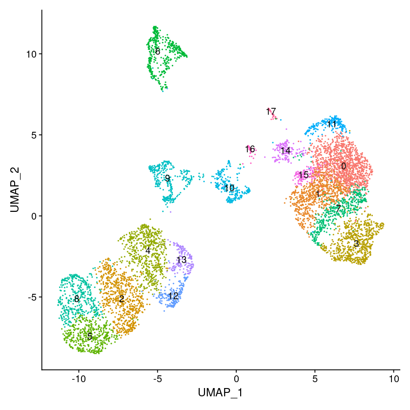
# Find clusters, then run UMAP, and visualize
pbmc <- FindNeighbors(pbmc, reduction = "peakvi", dims=1:ndims)
pbmc <- FindClusters(pbmc, resolution = 1)

pbmc <- RunUMAP(pbmc, reduction = "peakvi", dims=1:ndims)

options(repr.plot.width=7, repr.plot.height=7)
DimPlot(object = pbmc, label = TRUE) + NoLegend()
Computing nearest neighbor graph

Computing SNN
Modularity Optimizer version 1.3.0 by Ludo Waltman and Nees Jan van Eck

Number of nodes: 7060
Number of edges: 220834

Running Louvain algorithm...
Maximum modularity in 10 random starts: 0.8544
Number of communities: 18
Elapsed time: 0 seconds
Warning message:
"The default method for RunUMAP has changed from calling Python UMAP via reticulate to the R-native UWOT using the cosine metric
To use Python UMAP via reticulate, set umap.method to 'umap-learn' and metric to 'correlation'
This message will be shown once per session"
14:53:51 UMAP embedding parameters a = 0.9922 b = 1.112

14:53:51 Read 7060 rows and found 17 numeric columns

14:53:51 Using Annoy for neighbor search, n_neighbors = 30

14:53:51 Building Annoy index with metric = cosine, n_trees = 50

0%   10   20   30   40   50   60   70   80   90   100%

[----|----|----|----|----|----|----|----|----|----|

*
*
*
*
*
*
*
*
*
*
*
*
*
*
*
*
*
*
*
*
*
*
*
*
*
*
*
*
*
*
*
*
*
*
*
*
*
*
*
*
*
*
*
*
*
*
*
*
*
*
|

14:53:52 Writing NN index file to temp file /tmp/RtmpIDkqBd/file41f83787c253

14:53:52 Searching Annoy index using 1 thread, search_k = 3000

14:53:53 Annoy recall = 100%

14:53:55 Commencing smooth kNN distance calibration using 1 thread

14:53:56 Initializing from normalized Laplacian + noise

14:53:57 Commencing optimization for 500 epochs, with 279420 positive edges

14:54:02 Optimization finished
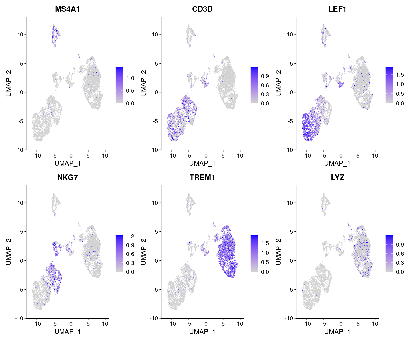
Create a gene activity matrix#
Important
The gene activity is used as an approximation of a gene expression matrix such that unpaired ATAC data can be integrated with RNA data. We recommend using this approach only for this unpaired case. Better results can be acheived if there is partially paired data, in which case MultiVI can be used.
[15]:
gene.activities <- GeneActivity(pbmc)

# add the gene activity matrix to the Seurat object as a new assay and normalize it
pbmc[['RNA']] <- CreateAssayObject(counts = gene.activities)
pbmc <- NormalizeData(
  object = pbmc,
  assay = 'RNA',
  normalization.method = 'LogNormalize',
  scale.factor = median(pbmc$nCount_RNA)
)
Extracting gene coordinates

Extracting reads overlapping genomic regions

Warning message:
"Non-unique features (rownames) present in the input matrix, making unique"
[16]:
options(repr.plot.width=12, repr.plot.height=10)

DefaultAssay(pbmc) <- 'RNA'

FeaturePlot(
  object = pbmc,
  features = c('MS4A1', 'CD3D', 'LEF1', 'NKG7', 'TREM1', 'LYZ'),
  pt.size = 0.1,
  max.cutoff = 'q95',
  ncol = 3
)
Integrating with scRNA-seq data (scANVI)#
We can integrate the gene activity matrix with annotated scRNA-seq data using scANVI.
First we download the Seurat-processed PBMC 10k dataset (as in their tutorial).
[23]:
system("wget https://www.dropbox.com/s/zn6khirjafoyyxl/pbmc_10k_v3.rds?dl=1 -O pbmc_10k_v3.rds")
[17]:
pbmc_rna <- readRDS("pbmc_10k_v3.rds")
And we convert it to AnnData using sceasy again. Subsequently, we follow the standard scANVI workflow: pretraining with scVI then running scANVI.
[18]:
adata_rna <- convertFormat(pbmc_rna, from="seurat", to="anndata", main_layer="counts", assay="RNA", drop_single_values=FALSE)
adata_atac_act <- convertFormat(pbmc, from="seurat", to="anndata", main_layer="counts", assay="RNA", drop_single_values=FALSE)

# provide adata_atac_act unknown cell type labels
adata_atac_act$obs$insert(adata_atac_act$obs$shape[1], "celltype", "Unknown")

adata_both <- adata_rna$concatenate(adata_atac_act)
None
We concatenated the RNA expression with the activity matrix using AnnData. Now we can see the last column is called “batch” and denotes which dataset each cell originated from.
[19]:
head(py_to_r(adata_both$obs))
| orig.ident | nCount_RNA | nFeature_RNA | observed | simulated | percent.mito | RNA_snn_res.0.4 | celltype | nCount_peaks | nFeature_peaks | ⋯ | peak_region_fragments | nucleosome_signal | nucleosome_percentile | TSS.enrichment | TSS.percentile | pct_reads_in_peaks | blacklist_ratio | peaks_snn_res.1 | seurat_clusters | batch | |
|---|---|---|---|---|---|---|---|---|---|---|---|---|---|---|---|---|---|---|---|---|---|
| <chr> | <dbl> | <int> | <dbl> | <dbl> | <dbl> | <fct> | <chr> | <dbl> | <dbl> | ⋯ | <dbl> | <dbl> | <dbl> | <dbl> | <dbl> | <dbl> | <dbl> | <fct> | <fct> | <fct> | |
| rna_AAACCCAAGCGCCCAT-1-0 | 10x_RNA | 2204 | 1087 | 0.035812672 | 0.4382022 | 0.02359347 | 1 | CD4 Memory | NaN | NaN | ⋯ | NaN | NaN | NaN | NaN | NaN | NaN | NaN | NA | NA | 0 |
| rna_AAACCCACAGAGTTGG-1-0 | 10x_RNA | 5884 | 1836 | 0.019227034 | 0.1017964 | 0.10757988 | 0 | CD14+ Monocytes | NaN | NaN | ⋯ | NaN | NaN | NaN | NaN | NaN | NaN | NaN | NA | NA | 0 |
| rna_AAACCCACAGGTATGG-1-0 | 10x_RNA | 5530 | 2216 | 0.005447865 | 0.1392801 | 0.07848101 | 5 | NK dim | NaN | NaN | ⋯ | NaN | NaN | NaN | NaN | NaN | NaN | NaN | NA | NA | 0 |
| rna_AAACCCACATAGTCAC-1-0 | 10x_RNA | 5106 | 1615 | 0.014276003 | 0.4949495 | 0.10830396 | 3 | pre-B cell | NaN | NaN | ⋯ | NaN | NaN | NaN | NaN | NaN | NaN | NaN | NA | NA | 0 |
| rna_AAACCCACATCCAATG-1-0 | 10x_RNA | 4572 | 1800 | 0.053857351 | 0.1392801 | 0.08989501 | 5 | NK bright | NaN | NaN | ⋯ | NaN | NaN | NaN | NaN | NaN | NaN | NaN | NA | NA | 0 |
| rna_AAACCCAGTGGCTACC-1-0 | 10x_RNA | 6702 | 1965 | 0.056603774 | 0.3554328 | 0.06326470 | 1 | CD4 Memory | NaN | NaN | ⋯ | NaN | NaN | NaN | NaN | NaN | NaN | NaN | NA | NA | 0 |
[20]:
sc$pp$highly_variable_genes(
    adata_both,
    flavor="seurat_v3",
    n_top_genes=r_to_py(3000),
    batch_key="batch",
    subset=TRUE
)
scvi$model$SCVI$setup_anndata(adata_both, labels_key="celltype", batch_key="batch")
None
None
[21]:
model <- scvi$model$SCVI(adata_both, gene_likelihood="nb", dispersion="gene-batch")
model$train()
None
[22]:
lvae <- scvi$model$SCANVI$from_scvi_model(model, "Unknown", adata=adata_both)
lvae$train(max_epochs = as.integer(100), n_samples_per_label = as.integer(100))
None
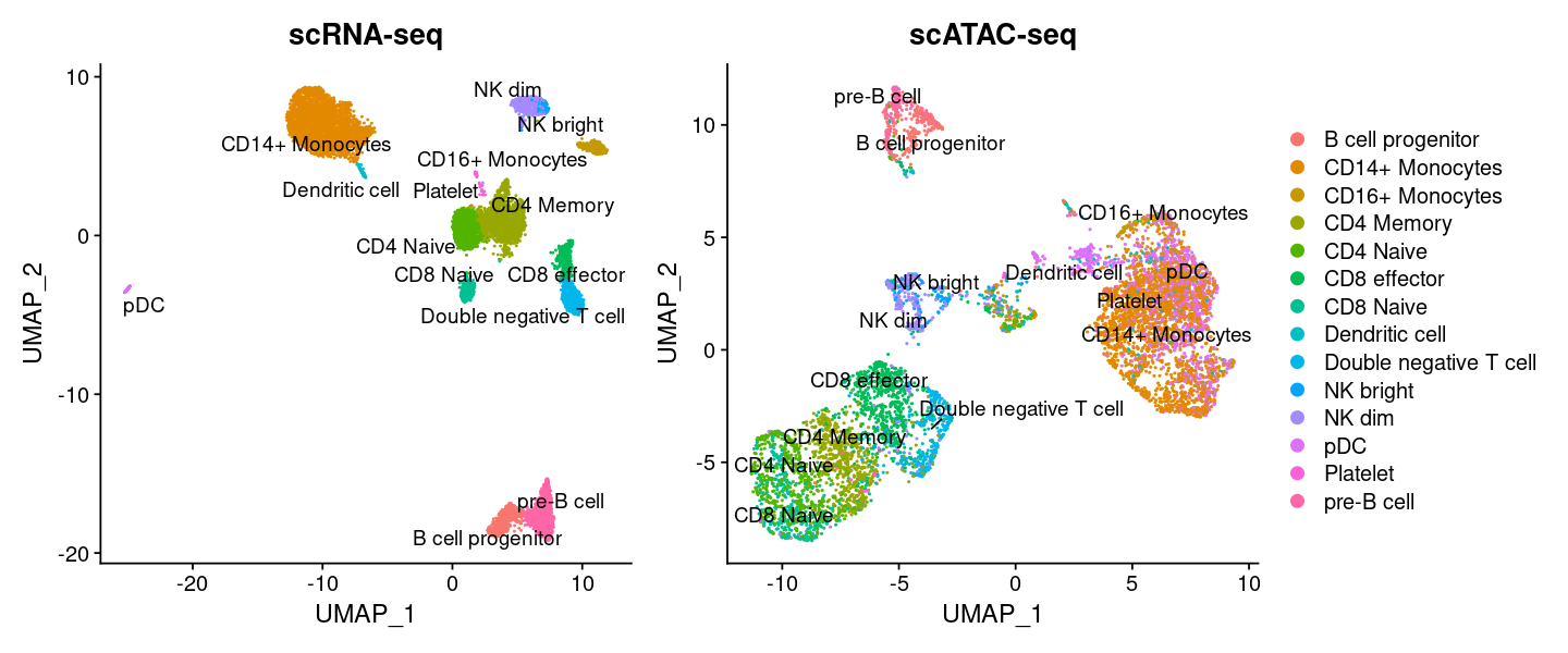
Here we only use the prediction functionality of scANVI, but we also could have viewed an integrated representation of the ATAC and RNA using UMAP.
[23]:
adata_both$obs$insert(adata_both$obs$shape[1], "predicted.labels", lvae$predict())
df <- py_to_r(adata_both$obs)
df <- subset(df, batch == 1)[, c("predicted.labels")]
pbmc <- AddMetaData(object = pbmc, metadata = df, col.name="predicted.labels")
None
Important
These labels should only serve as a starting point. Further inspection should always be performed. We leave this to the user, but will continue with these labels as a demonstration.
[24]:
options(repr.plot.width=12, repr.plot.height=5)

plot1 <- DimPlot(
  object = pbmc_rna,
  group.by = 'celltype',
  label = TRUE,
  repel = TRUE) + NoLegend() + ggtitle('scRNA-seq')

plot2 <- DimPlot(
  object = pbmc,
  group.by = 'predicted.labels',
  label = TRUE,
  repel = TRUE) + ggtitle('scATAC-seq')

plot1 + plot2
Finding differentially accessible peaks between clusters#
As PeakVI learns uncertainty around the observed data, it can be leveraged for differential accessibility analysis. First, let’s store the seurat cluster information back inside the AnnData.
[25]:
adata$obs$insert(adata$obs$shape[1], "predicted_ct", pbmc[["predicted.labels"]][,1])
None
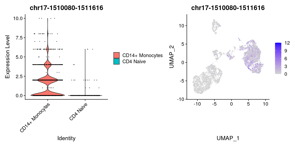
Using our trained PEAKVI model, we call the differential_accessibility() (DA) method We pass predicted_ct to the groupby argument and compare between naive CD4s and CD14 monocytes.
The output of DA is a DataFrame with the bayes factors. Bayes factors > 3 have high probability of being differentially expressed. You can also set fdr_target, which will return the differentially expressed genes based on the posteior expected FDR.
[26]:
DA <- pvi$differential_accessibility(adata, groupby="predicted_ct", group1 = "CD4 Naive", group2 = "CD14+ Monocytes")
DA <- py_to_r(DA)
head(DA)
| prob_da | is_da_fdr | bayes_factor | effect_size | emp_effect | est_prob1 | est_prob2 | emp_prob1 | emp_prob2 | |
|---|---|---|---|---|---|---|---|---|---|
| <dbl> | <lgl> | <dbl> | <dbl> | <dbl> | <dbl> | <dbl> | <dbl> | <dbl> | |
| chr1-565107-565550 | 0.0738 | FALSE | -2.5297313 | -0.02128995 | -0.009461094 | 0.03177977 | 0.010489821 | 0.014539580 | 0.005078486 |
| chr1-569174-569639 | 0.5342 | FALSE | 0.1370139 | -0.06247292 | -0.026307585 | 0.08119156 | 0.018718639 | 0.035541195 | 0.009233610 |
| chr1-713460-714823 | 0.9208 | TRUE | 2.4532664 | -0.27283466 | -0.164037549 | 0.73534369 | 0.462509036 | 0.389337641 | 0.225300092 |
| chr1-752422-753038 | 0.9722 | TRUE | 3.5545252 | 0.18390924 | 0.093491423 | 0.01899158 | 0.202900812 | 0.004846527 | 0.098337950 |
| chr1-762106-763359 | 0.8202 | FALSE | 1.5177030 | -0.15394741 | -0.096660536 | 0.51465970 | 0.360712290 | 0.266558966 | 0.169898430 |
| chr1-779589-780271 | 0.7834 | FALSE | 1.2855911 | -0.09098869 | -0.049387882 | 0.09661592 | 0.005627228 | 0.051696284 | 0.002308403 |
[27]:
# sort by proba_da and effect_size
DA <- DA[order(-DA[, 1], -DA[, 4]), ]
head(DA)
| prob_da | is_da_fdr | bayes_factor | effect_size | emp_effect | est_prob1 | est_prob2 | emp_prob1 | emp_prob2 | |
|---|---|---|---|---|---|---|---|---|---|
| <dbl> | <lgl> | <dbl> | <dbl> | <dbl> | <dbl> | <dbl> | <dbl> | <dbl> | |
| chr17-1510080-1511616 | 1.0000 | TRUE | 18.420681 | 0.8669005 | 0.4471439 | 0.04267091 | 0.90957141 | 0.027463651 | 0.474607572 |
| chr8-141108218-141111251 | 1.0000 | TRUE | 18.420681 | -0.8540915 | -0.4437980 | 0.89332950 | 0.03923802 | 0.466882068 | 0.023084026 |
| chr14-50504661-50507777 | 0.9998 | TRUE | 8.516943 | 0.8495569 | 0.5436486 | 0.14001995 | 0.98957688 | 0.085621971 | 0.629270545 |
| chr19-36397851-36401040 | 0.9998 | TRUE | 8.516943 | 0.8030195 | 0.3956684 | 0.07268646 | 0.87570596 | 0.035541195 | 0.431209603 |
| chr7-6674416-6675306 | 0.9998 | TRUE | 8.516943 | 0.4002175 | 0.1814427 | 0.01607980 | 0.41629726 | 0.009693053 | 0.191135734 |
| chr1-23945628-23947309 | 0.9998 | TRUE | 8.516943 | -0.7074655 | -0.3593336 | 0.72208506 | 0.01461957 | 0.366720517 | 0.007386888 |
[28]:
options(repr.plot.width=10, repr.plot.height=5)

DefaultAssay(pbmc) <- 'peaks'
Idents(pbmc) <- pbmc[["predicted.labels"]]

plot1 <- VlnPlot(
  object = pbmc,
  features = rownames(DA)[1],
  pt.size = 0.1,
  idents = c("CD4 Naive","CD14+ Monocytes")
)
plot2 <- FeaturePlot(
  object = pbmc,
  features = rownames(DA)[1],
  pt.size = 0.1
)

plot1 | plot2
[29]:
sI <- sessionInfo()
sI$loadedOnly <- NULL
print(sI, locale=FALSE)
R version 4.1.0 (2021-05-18)
Platform: x86_64-pc-linux-gnu (64-bit)
Running under: Ubuntu 20.04.2 LTS

Matrix products: default
BLAS:   /usr/lib/x86_64-linux-gnu/blas/libblas.so.3.9.0
LAPACK: /usr/lib/x86_64-linux-gnu/lapack/liblapack.so.3.9.0

attached base packages:
[1] stats4    stats     graphics  grDevices utils     datasets  methods
[8] base

other attached packages:
 [1] sceasy_0.0.6              reticulate_1.20
 [3] patchwork_1.1.1           ggplot2_3.3.5
 [5] EnsDb.Hsapiens.v75_2.99.0 ensembldb_2.17.4
 [7] AnnotationFilter_1.17.1   GenomicFeatures_1.45.2
 [9] AnnotationDbi_1.55.1      Biobase_2.53.0
[11] GenomicRanges_1.45.0      GenomeInfoDb_1.29.8
[13] IRanges_2.27.2            S4Vectors_0.31.3
[15] BiocGenerics_0.39.2       SeuratObject_4.0.2
[17] Seurat_4.0.4              Signac_1.3.0
[ ]: