Note
This page was generated from
totalVI.ipynb.
Interactive online version:
![]() .
Some tutorial content may look better in light mode.
.
Some tutorial content may look better in light mode.
CITE-seq analysis with totalVI#
With totalVI, we can produce a joint latent representation of cells, denoised data for both protein and RNA, integrate datasets, and compute differential expression of RNA and protein. Here we demonstrate this functionality with an integrated analysis of PBMC10k and PBMC5k, datasets of peripheral blood mononuclear cells publicly available from 10X Genomics subset to the 14 shared proteins between them. The same pipeline would generally be used to analyze a single CITE-seq dataset.
If you use totalVI, please consider citing:
Gayoso, A., Steier, Z., Lopez, R., Regier, J., Nazor, K. L., Streets, A., & Yosef, N. (2021). Joint probabilistic modeling of single-cell multi-omic data with totalVI. Nature Methods, 18(3), 272-282.
[1]:
!pip install --quiet scvi-colab
from scvi_colab import install
install()
Imports and data loading#
[2]:
import pandas as pd
import numpy as np
import matplotlib.pyplot as plt

import scvi
import scanpy as sc

sc.set_figure_params(figsize=(4, 4))

%config InlineBackend.print_figure_kwargs={'facecolor' : "w"}
%config InlineBackend.figure_format='retina'
Global seed set to 0
OMP: Info #276: omp_set_nested routine deprecated, please use omp_set_max_active_levels instead.
This dataset was filtered as described in the totalVI manuscript (low quality cells, doublets, lowly expressed genes, etc.)
[3]:
adata = scvi.data.pbmcs_10x_cite_seq()
adata.layers["counts"] = adata.X.copy()
sc.pp.normalize_total(adata, target_sum=1e4)
sc.pp.log1p(adata)
adata.raw = adata
INFO     File data/pbmc_10k_protein_v3.h5ad already downloaded
INFO     File data/pbmc_5k_protein_v3.h5ad already downloaded
Observation names are not unique. To make them unique, call `.obs_names_make_unique`.
[4]:
sc.pp.highly_variable_genes(
    adata,
    n_top_genes=4000,
    flavor="seurat_v3",
    batch_key="batch",
    subset=True,
    layer="counts"
)
Observation names are not unique. To make them unique, call `.obs_names_make_unique`.
Observation names are not unique. To make them unique, call `.obs_names_make_unique`.
[7]:
scvi.model.TOTALVI.setup_anndata(
    adata,
    protein_expression_obsm_key="protein_expression",
    layer="counts",
    batch_key="batch"
)
INFO Using column names from columns of adata.obsm['protein_expression']
Prepare and run model#
[8]:
vae = scvi.model.TOTALVI(adata, latent_distribution="normal")
INFO Computing empirical prior initialization for protein background.
[9]:
vae.train()
/data/yosef2/users/jhong/miniconda3/envs/v15/lib/python3.9/site-packages/torch/distributed/_sharded_tensor/__init__.py:8: DeprecationWarning: torch.distributed._sharded_tensor will be deprecated, use torch.distributed._shard.sharded_tensor instead
  warnings.warn(
GPU available: True, used: True
TPU available: False, using: 0 TPU cores
IPU available: False, using: 0 IPUs
LOCAL_RANK: 0 - CUDA_VISIBLE_DEVICES: [0,1,2]
Epoch 1/400: 0%| | 0/400 [00:00<?, ?it/s]
/data/yosef2/users/jhong/miniconda3/envs/v15/lib/python3.9/site-packages/scvi/distributions/_negative_binomial.py:97: UserWarning: Specified kernel cache directory could not be created! This disables kernel caching. Specified directory is /home/eecs/jjhong922/.cache/torch/kernels. This warning will appear only once per process. (Triggered internally at  /opt/conda/conda-bld/pytorch_1645690191318/work/aten/src/ATen/native/cuda/jit_utils.cpp:860.)
  + torch.lgamma(x + theta)
Epoch 322/400:  80%|████████  | 322/400 [06:16<01:28,  1.13s/it, loss=1.24e+03, v_num=1]Epoch 00322: reducing learning rate of group 0 to 2.4000e-03.
Epoch 367/400:  92%|█████████▏| 367/400 [07:07<00:37,  1.13s/it, loss=1.22e+03, v_num=1]Epoch 00367: reducing learning rate of group 0 to 1.4400e-03.
Epoch 400/400: 100%|██████████| 400/400 [07:45<00:00,  1.16s/it, loss=1.22e+03, v_num=1]
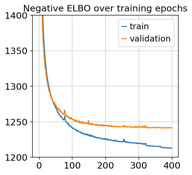
[10]:
plt.plot(vae.history["elbo_train"], label="train")
plt.plot(vae.history["elbo_validation"], label="validation")
plt.title("Negative ELBO over training epochs")
plt.ylim(1200, 1400)
plt.legend()
[10]:
<matplotlib.legend.Legend at 0x7f93ffdb8040>
Analyze outputs#
We use Scanpy for clustering and visualization after running totalVI. It’s also possible to save totalVI outputs for an R-based workflow. First, we store the totalVI outputs in the appropriate slots in AnnData.
[11]:
adata.obsm["X_totalVI"] = vae.get_latent_representation()

rna, protein = vae.get_normalized_expression(
    n_samples=25,
    return_mean=True,
    transform_batch=["PBMC10k", "PBMC5k"]
)

adata.layers["denoised_rna"], adata.obsm["denoised_protein"] = rna, protein

adata.obsm["protein_foreground_prob"] = vae.get_protein_foreground_probability(
    n_samples=25,
    return_mean=True,
    transform_batch=["PBMC10k", "PBMC5k"]
)
parsed_protein_names = [p.split("_")[0] for p in adata.obsm["protein_expression"].columns]
adata.obsm["protein_foreground_prob"].columns = parsed_protein_names
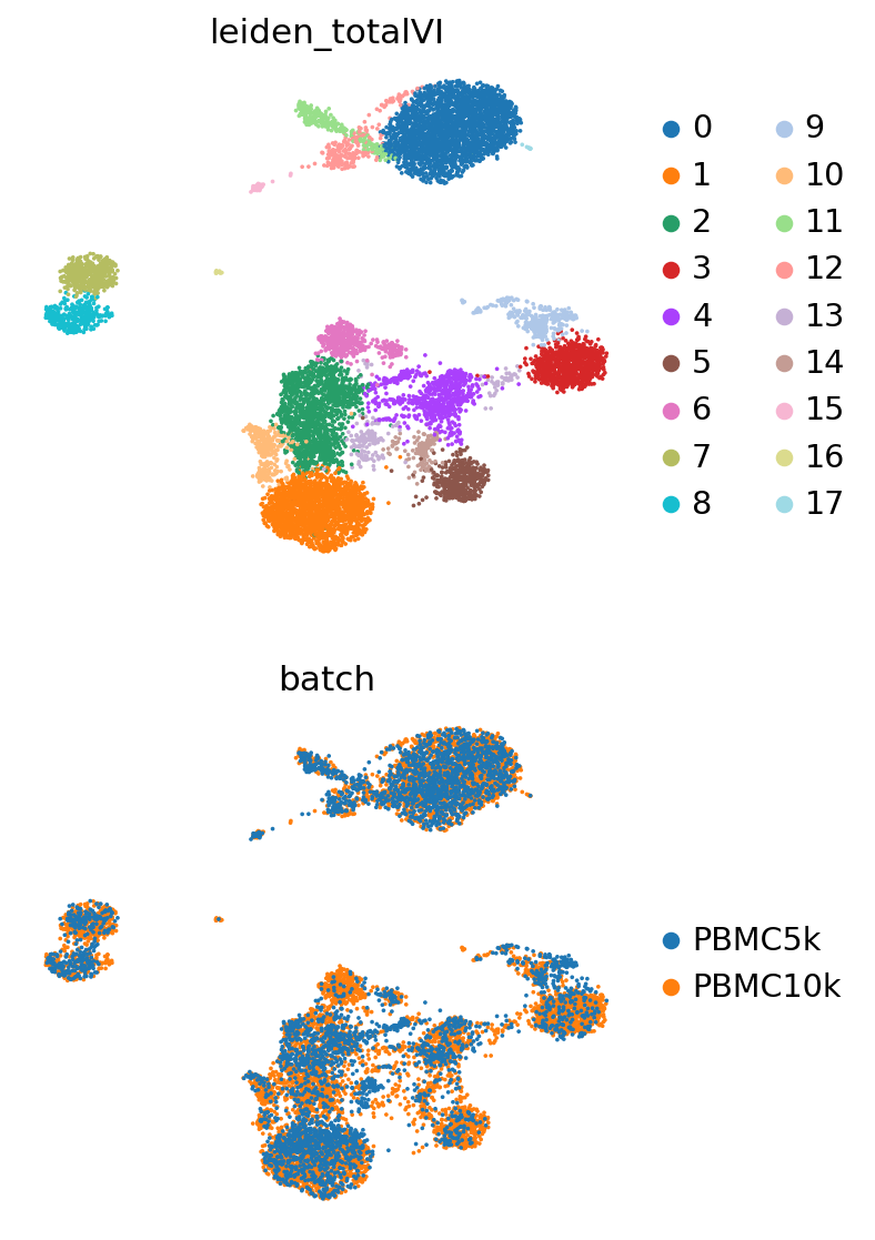
Now we can compute clusters and visualize the latent space.
[12]:
sc.pp.neighbors(adata, use_rep="X_totalVI")
sc.tl.umap(adata, min_dist=0.4)
sc.tl.leiden(adata, key_added="leiden_totalVI")
[13]:
sc.pl.umap(
    adata,
    color=["leiden_totalVI", "batch"],
    frameon=False,
    ncols=1,
)
/data/yosef2/users/jhong/miniconda3/envs/v15/lib/python3.9/site-packages/anndata/_core/anndata.py:1228: FutureWarning: The `inplace` parameter in pandas.Categorical.reorder_categories is deprecated and will be removed in a future version. Reordering categories will always return a new Categorical object.
  c.reorder_categories(natsorted(c.categories), inplace=True)
... storing 'batch' as categorical
To visualize protein values on the umap, we make a temporary protein adata object. We have to copy over the umap from the original adata object.
[14]:
pro_adata = sc.AnnData(adata.obsm["protein_expression"].copy(), obs=adata.obs)
sc.pp.log1p(pro_adata)
# Keep log normalized data in raw
pro_adata.raw = pro_adata
pro_adata.X = adata.obsm["denoised_protein"]
# these are cleaner protein names -- "_TotalSeqB" removed
pro_adata.var["protein_names"] = parsed_protein_names
pro_adata.obsm["X_umap"] = adata.obsm["X_umap"]
pro_adata.obsm["X_totalVI"] = adata.obsm["X_totalVI"]
Observation names are not unique. To make them unique, call `.obs_names_make_unique`.
[15]:
names = adata.obsm["protein_foreground_prob"].columns
for p in names:
    pro_adata.obs["{}_fore_prob".format(p)] = adata.obsm["protein_foreground_prob"].loc[:, p]
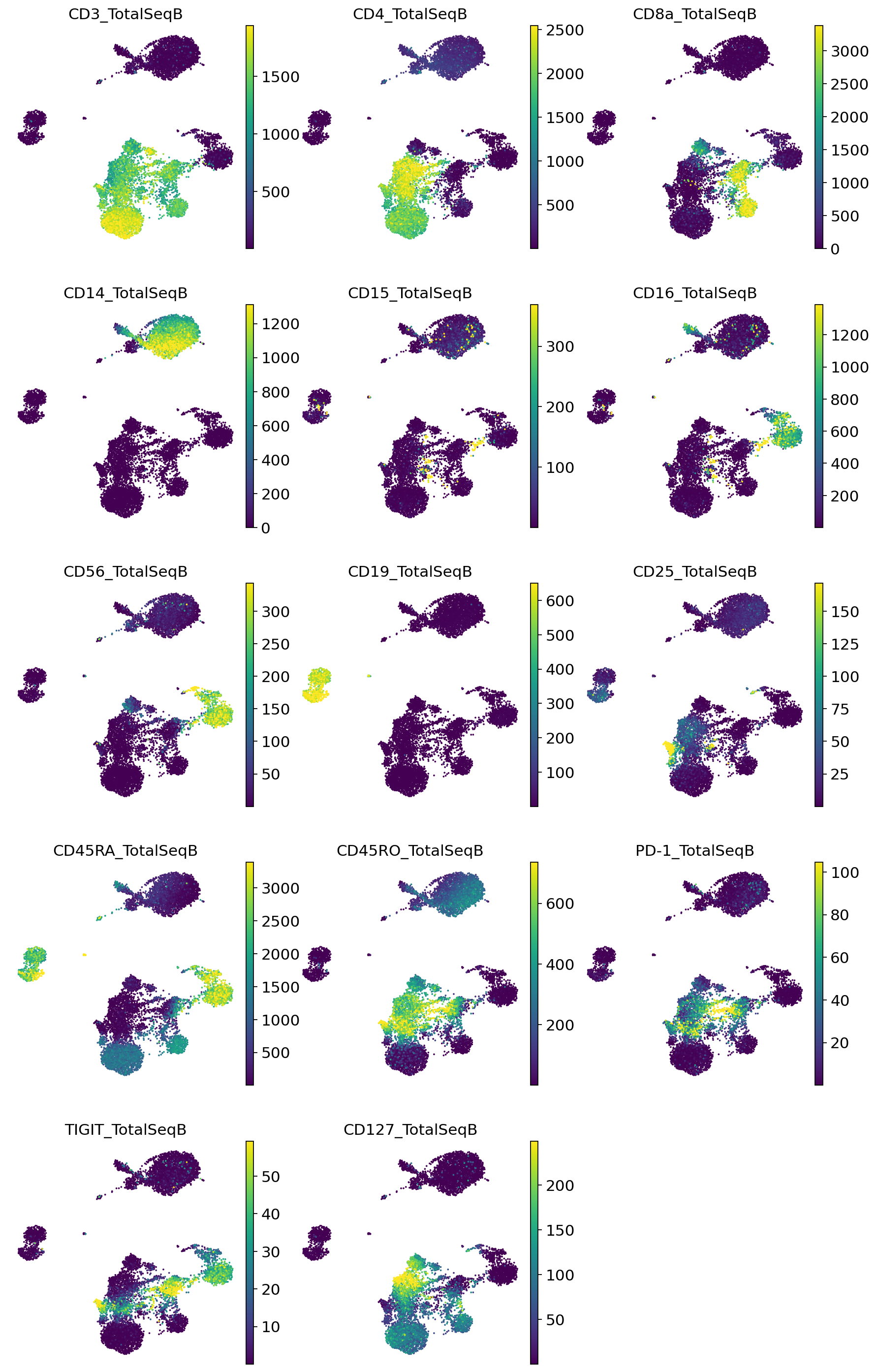
Visualize denoised protein values#
[16]:
sc.pl.umap(
    pro_adata,
    color=pro_adata.var_names,
    gene_symbols="protein_names",
    ncols=3,
    vmax="p99",
    use_raw=False,
    frameon=False,
    wspace=0.1
)
/data/yosef2/users/jhong/miniconda3/envs/v15/lib/python3.9/site-packages/scanpy/plotting/_tools/scatterplots.py:444: MatplotlibDeprecationWarning: Auto-removal of grids by pcolor() and pcolormesh() is deprecated since 3.5 and will be removed two minor releases later; please call grid(False) first.
  pl.colorbar(cax, ax=ax, pad=0.01, fraction=0.08, aspect=30)
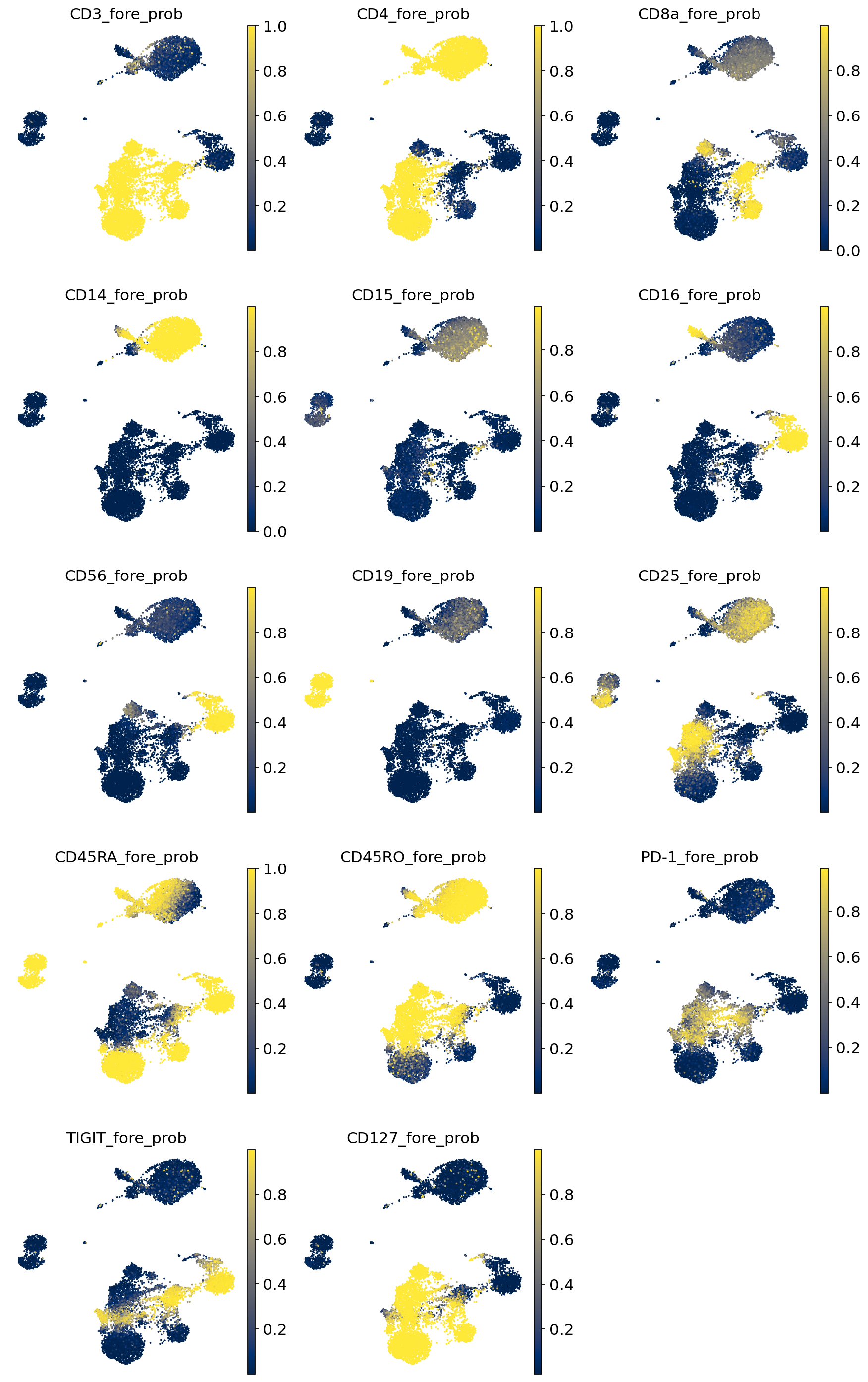
Visualize probability of foreground#
Here we visualize the probability of foreground for each protein and cell (projected on UMAP). Some proteins are easier to disentangle than others. Some proteins end up being “all background”. For example, CD15 does not appear to be captured well, when looking at the denoised values above we see little localization in the monocytes.
Note
While the foreground probability could theoretically be used to identify cell populations, we recommend using the denoised protein expression, which accounts for the foreground/background probability, but preserves the dynamic range of the protein measurements. Consequently, the denoised values are on the same scale as the raw data and it may be desirable to take a transformation like log or square root.
By viewing the foreground probability, we can get a feel for the types of cells in our dataset. For example, it’s very easy to see a population of monocytes based on the CD14 foregroud probability.
[17]:
sc.pl.umap(
    pro_adata,
    color=["{}_fore_prob".format(p) for p in parsed_protein_names],
    ncols=3,
    color_map="cividis",
    frameon=False,
    wspace=0.1
)
Differential expression#
Here we do a one-vs-all DE test, where each cluster is tested against all cells not in that cluster. The results for each of the one-vs-all tests is concatenated into one DataFrame object. Inividual tests can be sliced using the “comparison” column. Genes and proteins are included in the same DataFrame.
Important
We do not recommend using totalVI denoised values in other differential expression tools, as denoised values are a summary of a random quantity. The totalVI DE test takes into account the full uncertainty of the denoised quantities.
[18]:
de_df = vae.differential_expression(
        groupby="leiden_totalVI",
        delta=0.5,
        batch_correction=True
)
de_df.head(5)
DE...: 100%|██████████| 18/18 [00:51<00:00, 2.84s/it]
[18]:
| proba_de | proba_not_de | bayes_factor | scale1 | scale2 | pseudocounts | delta | lfc_mean | lfc_median | lfc_std | ... | raw_mean1 | raw_mean2 | non_zeros_proportion1 | non_zeros_proportion2 | raw_normalized_mean1 | raw_normalized_mean2 | is_de_fdr_0.05 | comparison | group1 | group2 | |
|---|---|---|---|---|---|---|---|---|---|---|---|---|---|---|---|---|---|---|---|---|---|
| WLS | 0.9990 | 0.0010 | 6.906745 | 0.000053 | 3.826878e-07 | 0.0 | 0.5 | 8.946897 | 9.093779 | 2.319537 | ... | 0.144357 | 0.001589 | 0.124484 | 0.001589 | 0.497803 | 0.003369 | True | 0 vs Rest | 0 | Rest |
| S100A12 | 0.9988 | 0.0012 | 6.724225 | 0.003306 | 2.673053e-05 | 0.0 | 0.5 | 8.952673 | 9.097330 | 2.377829 | ... | 9.262467 | 0.073943 | 0.944882 | 0.027255 | 34.482307 | 0.228318 | True | 0 vs Rest | 0 | Rest |
| ALDH1A1 | 0.9986 | 0.0014 | 6.569875 | 0.000246 | 2.337148e-06 | 0.0 | 0.5 | 8.541307 | 8.669662 | 2.453426 | ... | 0.661417 | 0.005378 | 0.394076 | 0.004522 | 2.366598 | 0.019742 | True | 0 vs Rest | 0 | Rest |
| C9ORF47 | 0.9986 | 0.0014 | 6.569875 | 0.000020 | 1.645234e-07 | 0.0 | 0.5 | 7.950605 | 8.018548 | 2.285622 | ... | 0.058868 | 0.000122 | 0.049119 | 0.000122 | 0.197639 | 0.000493 | True | 0 vs Rest | 0 | Rest |
| MARC1 | 0.9984 | 0.0016 | 6.436144 | 0.000119 | 8.664902e-07 | 0.0 | 0.5 | 8.722045 | 8.836887 | 2.555686 | ... | 0.302962 | 0.002322 | 0.234721 | 0.002078 | 1.172208 | 0.007004 | True | 0 vs Rest | 0 | Rest |
5 rows × 22 columns
Now we filter the results such that we retain features above a certain Bayes factor (which here is on the natural log scale) and genes with greater than 10% non-zero entries in the cluster of interest.
[19]:
filtered_pro = {}
filtered_rna = {}
cats = adata.obs.leiden_totalVI.cat.categories
for i, c in enumerate(cats):
    cid = "{} vs Rest".format(c)
    cell_type_df = de_df.loc[de_df.comparison == cid]
    cell_type_df = cell_type_df.sort_values("lfc_median", ascending=False)

    cell_type_df = cell_type_df[cell_type_df.lfc_median > 0]

    pro_rows = cell_type_df.index.str.contains('TotalSeqB')
    data_pro = cell_type_df.iloc[pro_rows]
    data_pro = data_pro[data_pro["bayes_factor"] > 0.7]

    data_rna = cell_type_df.iloc[~pro_rows]
    data_rna = data_rna[data_rna["bayes_factor"] > 3]
    data_rna = data_rna[data_rna["non_zeros_proportion1"] > 0.1]

    filtered_pro[c] = data_pro.index.tolist()[:3]
    filtered_rna[c] = data_rna.index.tolist()[:2]
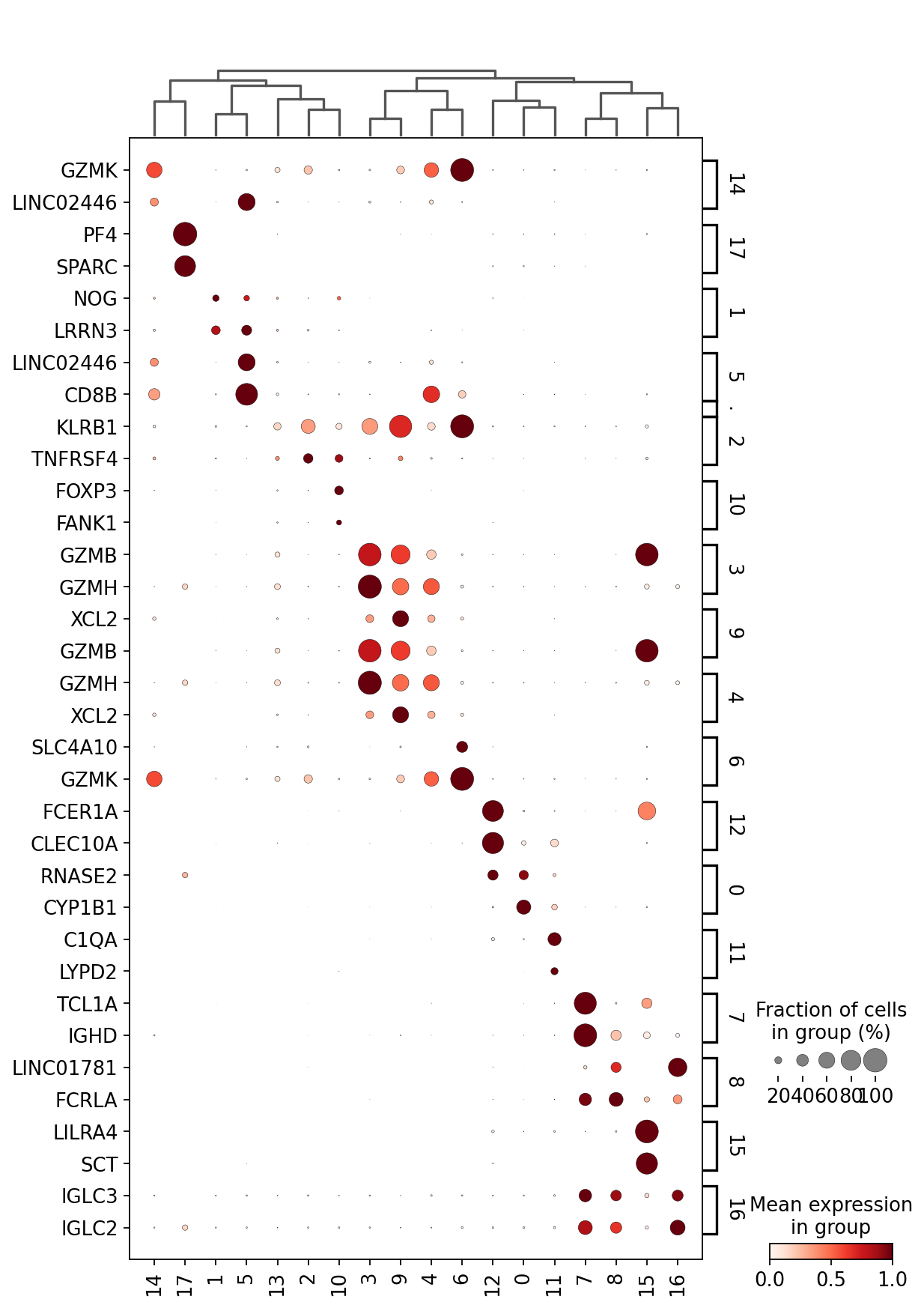
We can also use general scanpy visualization functions
[20]:
sc.tl.dendrogram(adata, groupby="leiden_totalVI", use_rep="X_totalVI")
sc.tl.dendrogram(pro_adata, groupby="leiden_totalVI", use_rep="X_totalVI")
[21]:
sc.pl.dotplot(
    adata,
    filtered_rna,
    groupby="leiden_totalVI",
    dendrogram=True,
    standard_scale="var",
    swap_axes=True
)
/data/yosef2/users/jhong/miniconda3/envs/v15/lib/python3.9/site-packages/scanpy/plotting/_baseplot_class.py:510: MatplotlibDeprecationWarning: Auto-removal of grids by pcolor() and pcolormesh() is deprecated since 3.5 and will be removed two minor releases later; please call grid(False) first.
  matplotlib.colorbar.ColorbarBase(
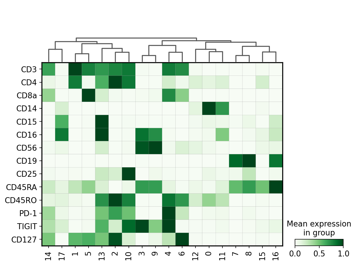
Matrix plot displays totalVI denoised protein expression per leiden cluster.
[22]:
sc.pl.matrixplot(
    pro_adata,
    pro_adata.var["protein_names"],
    groupby="leiden_totalVI",
    gene_symbols="protein_names",
    dendrogram=True,
    swap_axes=True,
    use_raw=False, # use totalVI denoised
    cmap="Greens",
    standard_scale="var"
)
/data/yosef2/users/jhong/miniconda3/envs/v15/lib/python3.9/site-packages/scanpy/plotting/_matrixplot.py:254: MatplotlibDeprecationWarning: Auto-removal of grids by pcolor() and pcolormesh() is deprecated since 3.5 and will be removed two minor releases later; please call grid(False) first.
  _ = ax.pcolor(_color_df, **kwds)
/data/yosef2/users/jhong/miniconda3/envs/v15/lib/python3.9/site-packages/scanpy/plotting/_baseplot_class.py:510: MatplotlibDeprecationWarning: Auto-removal of grids by pcolor() and pcolormesh() is deprecated since 3.5 and will be removed two minor releases later; please call grid(False) first.
  matplotlib.colorbar.ColorbarBase(
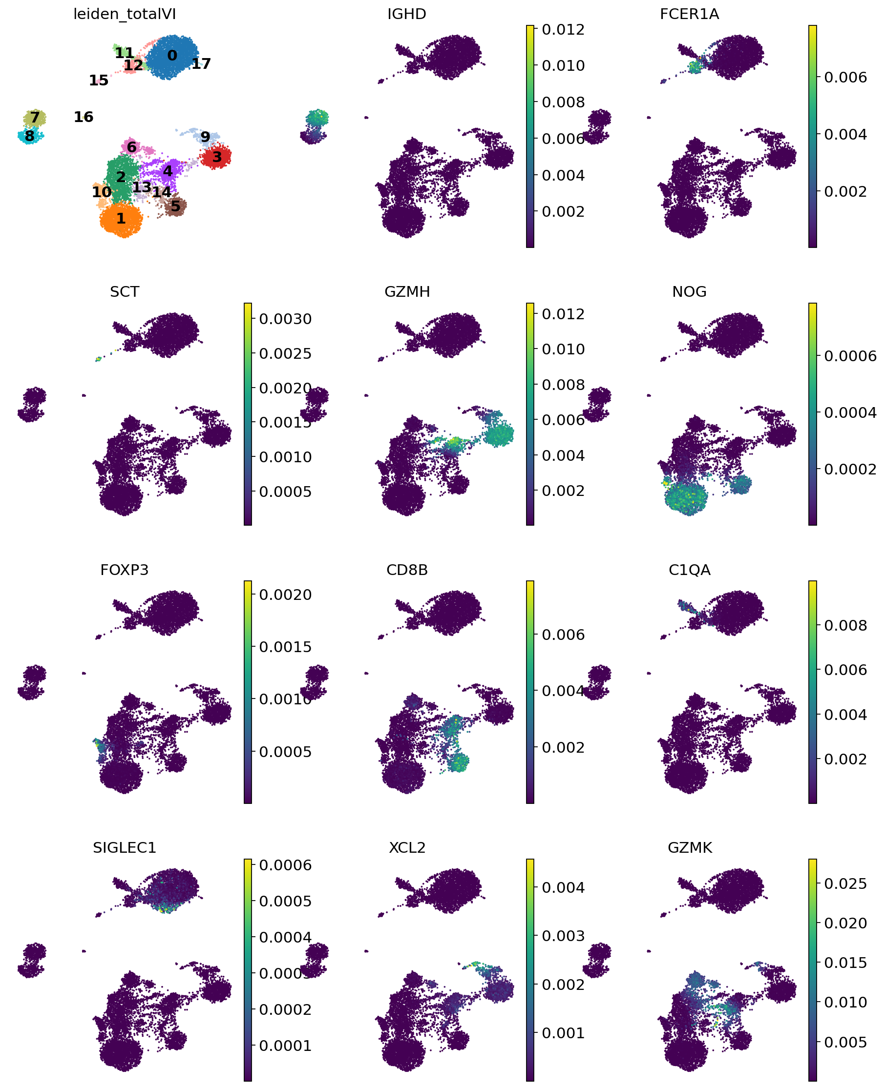
This is a selection of some of the markers that turned up in the RNA DE test.
[23]:
sc.pl.umap(
    adata,
    color=[
           "leiden_totalVI",
           "IGHD",
           "FCER1A",
           "SCT",
           "GZMH",
           "NOG",
           "FOXP3",
           "CD8B",
           "C1QA",
           "SIGLEC1",
           "XCL2",
           "GZMK",
           ],
    legend_loc="on data",
    frameon=False,
    ncols=3,
    layer="denoised_rna",
    wspace=0.1
)
/data/yosef2/users/jhong/miniconda3/envs/v15/lib/python3.9/site-packages/scanpy/plotting/_tools/scatterplots.py:444: MatplotlibDeprecationWarning: Auto-removal of grids by pcolor() and pcolormesh() is deprecated since 3.5 and will be removed two minor releases later; please call grid(False) first.
  pl.colorbar(cax, ax=ax, pad=0.01, fraction=0.08, aspect=30)