Note
This page was generated from
stereoscope_heart_LV_tutorial.ipynb.
Interactive online version:
![]() .
Some tutorial content may look better in light mode.
.
Some tutorial content may look better in light mode.
Stereoscope applied to left ventricule data#
Developed by Carlos Talavera-López Ph.D, WSI, edited by Romain Lopez
Version: 210301
In this notebook, we present the workflow to run Stereoscope within the scvi-tools codebase. We map the adult heart cell atlas data from Litviňuková et al (2020). This experiment takes around one hour to run on Colab.
You can access the raw count matrices as ‘anndata’ objects at www.heartcellatlas.org.
[ ]:
!pip install --quiet scvi-colab
from scvi_colab import install

install()
[1]:
import warnings

import matplotlib.pyplot as plt
import numpy as np
import scanpy as sc
import seaborn as sns
from scvi.external import RNAStereoscope, SpatialStereoscope
[2]:
warnings.filterwarnings("ignore")

%matplotlib inline
%config InlineBackend.print_figure_kwargs={'facecolor' : "w"}
%config InlineBackend.figure_format='retina'
Global seed set to 0
OMP: Info #276: omp_set_nested routine deprecated, please use omp_set_max_active_levels instead.
Download and preprocess data#
[3]:
!wget -O hca_heart_LV_stereoscope_subset_raw_ctl201217.h5ad https://ndownloader.figshare.com/files/26153564
--2022-02-26 15:13:06--  https://ndownloader.figshare.com/files/26153564
Resolving ndownloader.figshare.com (ndownloader.figshare.com)... 52.16.102.173, 54.217.124.219, 2a05:d018:1f4:d003:1c8b:1823:acce:812, ...
Connecting to ndownloader.figshare.com (ndownloader.figshare.com)|52.16.102.173|:443... connected.
HTTP request sent, awaiting response... 302 Found
Location: https://s3-eu-west-1.amazonaws.com/pfigshare-u-files/26153564/hca_heart_LV_stereoscope_subset_raw_ctl201217.h5ad?X-Amz-Algorithm=AWS4-HMAC-SHA256&X-Amz-Credential=AKIAIYCQYOYV5JSSROOA/20220226/eu-west-1/s3/aws4_request&X-Amz-Date=20220226T231307Z&X-Amz-Expires=10&X-Amz-SignedHeaders=host&X-Amz-Signature=37396458be74605c30c79c368a37fc6ea412c010249e24c15d3cfef09ebdfb31 [following]
--2022-02-26 15:13:07--  https://s3-eu-west-1.amazonaws.com/pfigshare-u-files/26153564/hca_heart_LV_stereoscope_subset_raw_ctl201217.h5ad?X-Amz-Algorithm=AWS4-HMAC-SHA256&X-Amz-Credential=AKIAIYCQYOYV5JSSROOA/20220226/eu-west-1/s3/aws4_request&X-Amz-Date=20220226T231307Z&X-Amz-Expires=10&X-Amz-SignedHeaders=host&X-Amz-Signature=37396458be74605c30c79c368a37fc6ea412c010249e24c15d3cfef09ebdfb31
Resolving s3-eu-west-1.amazonaws.com (s3-eu-west-1.amazonaws.com)... 52.218.65.44
Connecting to s3-eu-west-1.amazonaws.com (s3-eu-west-1.amazonaws.com)|52.218.65.44|:443... connected.
HTTP request sent, awaiting response... 200 OK
Length: 130445704 (124M) [application/octet-stream]
Saving to: ‘hca_heart_LV_stereoscope_subset_raw_ctl201217.h5ad’

hca_heart_LV_stereo 100%[===================>] 124.40M  3.59MB/s    in 37s

2022-02-26 15:13:45 (3.33 MB/s) - ‘hca_heart_LV_stereoscope_subset_raw_ctl201217.h5ad’ saved [130445704/130445704]
Read in single-cell data#
Read in expression data. This is a subset of the data you want to map. Here I use a balanced subset of cells from the left ventricle (~ 50K). You can create your own subset according to what you are interested in.
[4]:
sc_adata = sc.read_h5ad("hca_heart_LV_stereoscope_subset_raw_ctl201217.h5ad")
sc_adata
[4]:
AnnData object with n_obs × n_vars = 35928 × 33538
    obs: 'age_group', 'cell_source', 'cell_type', 'donor', 'gender', 'n_counts', 'n_genes', 'percent_mito', 'percent_ribo', 'region', 'sample', 'scrublet_score', 'version', 'cell_states'
    var: 'gene_ids-Harvard-Nuclei', 'feature_types-Harvard-Nuclei', 'gene_ids-Sanger-Nuclei', 'feature_types-Sanger-Nuclei', 'gene_ids-Sanger-Cells', 'feature_types-Sanger-Cells', 'gene_ids-Sanger-CD45', 'feature_types-Sanger-CD45'
    obsm: 'X_pca', 'X_umap'
[5]:
sc.pp.filter_genes(sc_adata, min_counts=10)
sc_adata
[5]:
AnnData object with n_obs × n_vars = 35928 × 25145
    obs: 'age_group', 'cell_source', 'cell_type', 'donor', 'gender', 'n_counts', 'n_genes', 'percent_mito', 'percent_ribo', 'region', 'sample', 'scrublet_score', 'version', 'cell_states'
    var: 'gene_ids-Harvard-Nuclei', 'feature_types-Harvard-Nuclei', 'gene_ids-Sanger-Nuclei', 'feature_types-Sanger-Nuclei', 'gene_ids-Sanger-Cells', 'feature_types-Sanger-Cells', 'gene_ids-Sanger-CD45', 'feature_types-Sanger-CD45', 'n_counts'
    obsm: 'X_pca', 'X_umap'
[6]:
sc_adata.obs["combined"] = [
    sc_adata.obs.loc[i, "cell_source"] + sc_adata.obs.loc[i, "donor"]
    for i in sc_adata.obs_names
]
sc_adata
[6]:
AnnData object with n_obs × n_vars = 35928 × 25145
    obs: 'age_group', 'cell_source', 'cell_type', 'donor', 'gender', 'n_counts', 'n_genes', 'percent_mito', 'percent_ribo', 'region', 'sample', 'scrublet_score', 'version', 'cell_states', 'combined'
    var: 'gene_ids-Harvard-Nuclei', 'feature_types-Harvard-Nuclei', 'gene_ids-Sanger-Nuclei', 'feature_types-Sanger-Nuclei', 'gene_ids-Sanger-Cells', 'feature_types-Sanger-Cells', 'gene_ids-Sanger-CD45', 'feature_types-Sanger-CD45', 'n_counts'
    obsm: 'X_pca', 'X_umap'
Remove mitochondrial genes
[7]:
non_mito_genes_list = [
    name for name in sc_adata.var_names if not name.startswith("MT-")
]
sc_adata = sc_adata[:, non_mito_genes_list]
sc_adata
[7]:
View of AnnData object with n_obs × n_vars = 35928 × 25132
    obs: 'age_group', 'cell_source', 'cell_type', 'donor', 'gender', 'n_counts', 'n_genes', 'percent_mito', 'percent_ribo', 'region', 'sample', 'scrublet_score', 'version', 'cell_states', 'combined'
    var: 'gene_ids-Harvard-Nuclei', 'feature_types-Harvard-Nuclei', 'gene_ids-Sanger-Nuclei', 'feature_types-Sanger-Nuclei', 'gene_ids-Sanger-Cells', 'feature_types-Sanger-Cells', 'gene_ids-Sanger-CD45', 'feature_types-Sanger-CD45', 'n_counts'
    obsm: 'X_pca', 'X_umap'
Normalize data on a different layer, because Stereoscope works with raw counts. We did not see better results by using all the genes, so for computational purposed we cut here to 7,000 genes.
[8]:
sc_adata.layers["counts"] = sc_adata.X.copy()
sc.pp.normalize_total(sc_adata, target_sum=1e5)
sc.pp.log1p(sc_adata)
sc_adata.raw = sc_adata
[9]:
sc.pp.highly_variable_genes(
    sc_adata,
    n_top_genes=7000,
    subset=True,
    layer="counts",
    flavor="seurat_v3",
    batch_key="combined",
    span=1,
)
Examine the cell type labels
[10]:
sc_adata.obs["cell_states"].value_counts()
[10]:
EC5_art        2000
PC3_str        2000
EC2_cap        2000
EC1_cap        2000
vCM1           2000
FB1            2000
SMC1_basic     2000
PC1_vent       2000
vCM2           2000
vCM3           2000
vCM4           2000
FB4            1912
EC3_cap        1712
EC6_ven        1292
DOCK4+MØ1       970
EC4_immune      751
CD4+T_cytox     642
NC1             524
Mast            453
FB3             436
CD8+T_cytox     429
LYVE1+MØ1       394
LYVE1+MØ2       390
CD8+T_tem       368
SMC2_art        323
NK              322
FB2             308
FB5             245
vCM5            235
CD16+Mo         234
Mo_pi           227
NKT             224
LYVE1+MØ3       223
CD4+T_tem       170
DC              143
CD14+Mo         132
Adip1           126
MØ_AgP          116
B_cells         112
NC2             102
DOCK4+MØ2        99
EC8_ln           90
NC4              59
MØ_mod           48
NC3              39
Meso             30
Adip2            15
Adip4            11
Adip3             8
NØ                7
IL17RA+Mo         3
NC5               2
NC6               2
Name: cell_states, dtype: int64
Read in visium data#
[11]:
st_adata = sc.datasets.visium_sge(sample_id="V1_Human_Heart")
st_adata.var_names_make_unique()
Variable names are not unique. To make them unique, call `.var_names_make_unique`.
Variable names are not unique. To make them unique, call `.var_names_make_unique`.
[12]:
st_adata.var["mt"] = st_adata.var_names.str.startswith("MT-")
sc.pp.calculate_qc_metrics(st_adata, qc_vars=["mt"], inplace=True)
st_adata
[12]:
AnnData object with n_obs × n_vars = 4235 × 33538
    obs: 'in_tissue', 'array_row', 'array_col', 'n_genes_by_counts', 'log1p_n_genes_by_counts', 'total_counts', 'log1p_total_counts', 'pct_counts_in_top_50_genes', 'pct_counts_in_top_100_genes', 'pct_counts_in_top_200_genes', 'pct_counts_in_top_500_genes', 'total_counts_mt', 'log1p_total_counts_mt', 'pct_counts_mt'
    var: 'gene_ids', 'feature_types', 'genome', 'mt', 'n_cells_by_counts', 'mean_counts', 'log1p_mean_counts', 'pct_dropout_by_counts', 'total_counts', 'log1p_total_counts'
    uns: 'spatial'
    obsm: 'spatial'
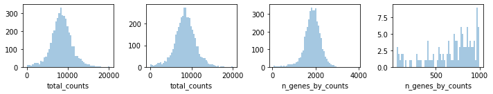
Clean up data based on QC values
[13]:
fig, axs = plt.subplots(1, 4, figsize=(10, 2))
sns.distplot(st_adata.obs["total_counts"], kde=False, ax=axs[0])
sns.distplot(
    st_adata.obs["total_counts"][st_adata.obs["total_counts"] < 20000],
    kde=False,
    bins=60,
    ax=axs[1],
)
sns.distplot(st_adata.obs["n_genes_by_counts"], kde=False, bins=60, ax=axs[2])
sns.distplot(
    st_adata.obs["n_genes_by_counts"][st_adata.obs["n_genes_by_counts"] < 1000],
    kde=False,
    bins=60,
    ax=axs[3],
)
plt.tight_layout()
plt.show()
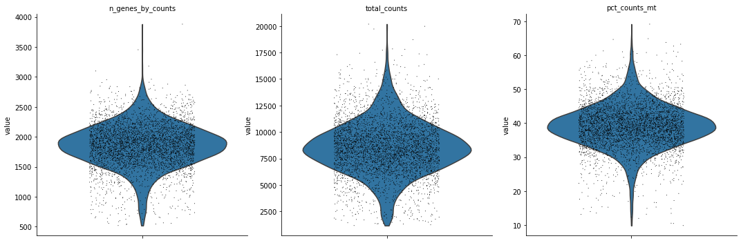
[14]:
sc.pp.filter_cells(st_adata, min_counts=500)
sc.pp.filter_cells(st_adata, min_genes=500)
sc.pl.violin(
    st_adata,
    ["n_genes_by_counts", "total_counts", "pct_counts_mt"],
    jitter=0.25,
    multi_panel=True,
)
st_adata
... storing 'feature_types' as categorical
... storing 'genome' as categorical
[14]:
AnnData object with n_obs × n_vars = 4206 × 33538
    obs: 'in_tissue', 'array_row', 'array_col', 'n_genes_by_counts', 'log1p_n_genes_by_counts', 'total_counts', 'log1p_total_counts', 'pct_counts_in_top_50_genes', 'pct_counts_in_top_100_genes', 'pct_counts_in_top_200_genes', 'pct_counts_in_top_500_genes', 'total_counts_mt', 'log1p_total_counts_mt', 'pct_counts_mt', 'n_counts', 'n_genes'
    var: 'gene_ids', 'feature_types', 'genome', 'mt', 'n_cells_by_counts', 'mean_counts', 'log1p_mean_counts', 'pct_dropout_by_counts', 'total_counts', 'log1p_total_counts'
    uns: 'spatial'
    obsm: 'spatial'
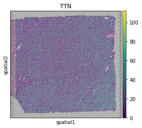
[15]:
sc.pl.spatial(st_adata, img_key="hires", color=["TTN"])
Learn cell-type specific gene expression from scRNA-seq data#
Filter genes to be the same on the spatial data
[16]:
intersect = np.intersect1d(sc_adata.var_names, st_adata.var_names)
st_adata = st_adata[:, intersect].copy()
sc_adata = sc_adata[:, intersect].copy()
Setup the AnnData object
[17]:
RNAStereoscope.setup_anndata(sc_adata, layer="counts", labels_key="cell_states")
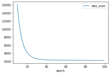
Train the scRNA-Seq model
[18]:
train = True
if train:
    sc_model = RNAStereoscope(sc_adata)
    sc_model.train(max_epochs=100)
    sc_model.history["elbo_train"][10:].plot()
    sc_model.save("scmodel", overwrite=True)
else:
    sc_model = RNAStereoscope.load("scmodel", adata=sc_adata)
    print("Loaded RNA model from file!")
GPU available: True, used: True
TPU available: False, using: 0 TPU cores
IPU available: False, using: 0 IPUs
LOCAL_RANK: 0 - CUDA_VISIBLE_DEVICES: [0,1,2]
Epoch 100/100: 100%|██████████| 100/100 [04:29<00:00, 2.69s/it, loss=2.79e+05, v_num=1]
Infer proportion for spatial data#
[19]:
st_adata.layers["counts"] = st_adata.X.copy()
SpatialStereoscope.setup_anndata(st_adata, layer="counts")
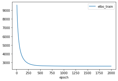
Train Visium model
[20]:
train = True
if train:
    spatial_model = SpatialStereoscope.from_rna_model(st_adata, sc_model)
    spatial_model.train(max_epochs=2000)
    spatial_model.history["elbo_train"][10:].plot()
    spatial_model.save("stmodel", overwrite=True)
else:
    spatial_model = SpatialStereoscope.load("stmodel", adata=st_adata)
    print("Loaded Spatial model from file!")
GPU available: True, used: True
TPU available: False, using: 0 TPU cores
IPU available: False, using: 0 IPUs
LOCAL_RANK: 0 - CUDA_VISIBLE_DEVICES: [0,1,2]
Epoch 2000/2000: 100%|██████████| 2000/2000 [10:56<00:00, 3.05it/s, loss=1.09e+07, v_num=1]
Deconvolution results#
[21]:
st_adata.obsm["deconvolution"] = spatial_model.get_proportions()

# also copy as single field in the anndata for visualization
for ct in st_adata.obsm["deconvolution"].columns:
    st_adata.obs[ct] = st_adata.obsm["deconvolution"][ct]
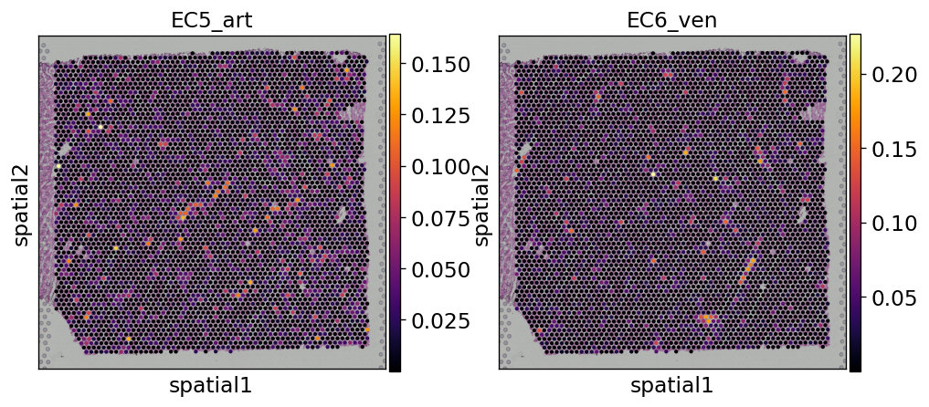
Visualise populations#
Et voilá, we have now an anndata object that contains the inferred proportions on each Visium spot for each cell type in our single cell reference dataset.
In this example we can observe how nicely the arterial endotehlial cells (EC5_art) and the venous endothelial cells (EC6_ven) are highlighted in the areas were we expect to see cardiac vessels based on the histology of the sample.
[22]:
# low dpi for uploading to github
sc.settings.set_figure_params(
    dpi=60, color_map="RdPu", dpi_save=200, vector_friendly=True, format="svg"
)
sc.pl.spatial(
    st_adata,
    img_key="hires",
    color=["EC5_art", "EC6_ven"],
    size=1.2,
    color_map="inferno",
)
[ ]: