Note

This page was generated from scbasset.ipynb. Interactive online version: . Some tutorial content may look better in light mode.

ScBasset: Analyzing scATACseq data#

Warning

SCBASSET’s development is still in progress. The current version may not fully reproduce the original implementation’s results.

[5]:

!pip install --quiet scvi-colab
from scvi_colab import install

install()

/home/adam/miniconda3/envs/scvi-tools-dev/lib/python3.10/site-packages/scvi_colab/_core.py:41: UserWarning:
                Not currently in Google Colab environment.

                Please run with `run_outside_colab=True` to override.

                Returning with no further action.

  warn(

[1]:

import matplotlib.pyplot as plt
import muon
import numpy as np
import scanpy as sc
import scvi
import seaborn as sns

Global seed set to 0

[2]:

scvi.settings.seed = 0

sc.set_figure_params(figsize=(4, 4), frameon=False)

%config InlineBackend.print_figure_kwargs={'facecolor' : "w"}
%config InlineBackend.figure_format='retina'

Global seed set to 0

Loading data and preprocessing#

Throughout this tutorial, we use sample multiome data from 10X of 10K PBMCs.

[3]:

url = "https://cf.10xgenomics.com/samples/cell-arc/2.0.0/10k_PBMC_Multiome_nextgem_Chromium_X/10k_PBMC_Multiome_nextgem_Chromium_X_filtered_feature_bc_matrix.h5"
mdata = muon.read_10x_h5("data/multiome10k.h5mu", backup_url=url)

/home/adam/miniconda3/envs/scvi-tools-dev/lib/python3.10/site-packages/anndata/_core/anndata.py:1830: UserWarning: Variable names are not unique. To make them unique, call `.var_names_make_unique`.
  utils.warn_names_duplicates("var")

Added `interval` annotation for features from data/multiome10k.h5mu

/home/adam/miniconda3/envs/scvi-tools-dev/lib/python3.10/site-packages/anndata/_core/anndata.py:1830: UserWarning: Variable names are not unique. To make them unique, call `.var_names_make_unique`.
  utils.warn_names_duplicates("var")
/home/adam/miniconda3/envs/scvi-tools-dev/lib/python3.10/site-packages/mudata/_core/mudata.py:446: UserWarning: var_names are not unique. To make them unique, call `.var_names_make_unique`.
  warnings.warn(

[4]:

mdata

[4]:

MuData object with n_obs × n_vars = 10970 × 148344
  var:      'gene_ids', 'feature_types', 'genome', 'interval'
  2 modalities
    rna:    10970 x 36601
      var:  'gene_ids', 'feature_types', 'genome', 'interval'
    atac:   10970 x 111743
      var:  'gene_ids', 'feature_types', 'genome', 'interval'

[5]:

adata = mdata.mod["atac"]

We can use scanpy functions to handle, filter, and manipulate the data. In our case, we might want to filter out peaks that are rarely detected, to make the model train faster:

[6]:

print(adata.shape)
# compute the threshold: 5% of the cells
min_cells = int(adata.shape[0] * 0.05)
# in-place filtering of regions
sc.pp.filter_genes(adata, min_cells=min_cells)
print(adata.shape)

(10970, 111743)
(10970, 37054)

[7]:

adata.var

[7]:

	gene_ids	feature_types	genome	interval	n_cells
chr1:629395-630394	chr1:629395-630394	Peaks	GRCh38	chr1:629395-630394	1422
chr1:633578-634591	chr1:633578-634591	Peaks	GRCh38	chr1:633578-634591	4536
chr1:778283-779200	chr1:778283-779200	Peaks	GRCh38	chr1:778283-779200	5981
chr1:816873-817775	chr1:816873-817775	Peaks	GRCh38	chr1:816873-817775	564
chr1:827067-827949	chr1:827067-827949	Peaks	GRCh38	chr1:827067-827949	3150
...	...	...	...	...	...
GL000219.1:44739-45583	GL000219.1:44739-45583	Peaks	GRCh38	GL000219.1:44739-45583	781
GL000219.1:45726-46446	GL000219.1:45726-46446	Peaks	GRCh38	GL000219.1:45726-46446	639
GL000219.1:99267-100169	GL000219.1:99267-100169	Peaks	GRCh38	GL000219.1:99267-100169	6830
KI270726.1:41483-42332	KI270726.1:41483-42332	Peaks	GRCh38	KI270726.1:41483-42332	605
KI270713.1:21453-22374	KI270713.1:21453-22374	Peaks	GRCh38	KI270713.1:21453-22374	6247

37054 rows × 5 columns

[8]:

split_interval = adata.var["gene_ids"].str.split(":", expand=True)
adata.var["chr"] = split_interval[0]
split_start_end = split_interval[1].str.split("-", expand=True)
adata.var["start"] = split_start_end[0].astype(int)
adata.var["end"] = split_start_end[1].astype(int)
adata.var

[8]:

	gene_ids	feature_types	genome	interval	n_cells	chr	start	end
chr1:629395-630394	chr1:629395-630394	Peaks	GRCh38	chr1:629395-630394	1422	chr1	629395	630394
chr1:633578-634591	chr1:633578-634591	Peaks	GRCh38	chr1:633578-634591	4536	chr1	633578	634591
chr1:778283-779200	chr1:778283-779200	Peaks	GRCh38	chr1:778283-779200	5981	chr1	778283	779200
chr1:816873-817775	chr1:816873-817775	Peaks	GRCh38	chr1:816873-817775	564	chr1	816873	817775
chr1:827067-827949	chr1:827067-827949	Peaks	GRCh38	chr1:827067-827949	3150	chr1	827067	827949
...	...	...	...	...	...	...	...	...
GL000219.1:44739-45583	GL000219.1:44739-45583	Peaks	GRCh38	GL000219.1:44739-45583	781	GL000219.1	44739	45583
GL000219.1:45726-46446	GL000219.1:45726-46446	Peaks	GRCh38	GL000219.1:45726-46446	639	GL000219.1	45726	46446
GL000219.1:99267-100169	GL000219.1:99267-100169	Peaks	GRCh38	GL000219.1:99267-100169	6830	GL000219.1	99267	100169
KI270726.1:41483-42332	KI270726.1:41483-42332	Peaks	GRCh38	KI270726.1:41483-42332	605	KI270726.1	41483	42332
KI270713.1:21453-22374	KI270713.1:21453-22374	Peaks	GRCh38	KI270713.1:21453-22374	6247	KI270713.1	21453	22374

37054 rows × 8 columns

[9]:

# Filter out non-chromosomal regions
mask = adata.var["chr"].str.startswith("chr")
adata = adata[:, mask].copy()

[14]:

scvi.data.add_dna_sequence(
    adata,
    genome_name="GRCh38",
    genome_dir="data",
    chr_var_key="chr",
    start_var_key="start",
    end_var_key="end",
)
adata

10:19:43 | INFO | Downloading genome from GENCODE. Target URL: http://hgdownload.soe.ucsc.edu/goldenPath/hg38/bigZips/hg38.fa.gz...

10:19:52 | INFO | Genome download successful, starting post processing...
10:20:02 | INFO | name: hg38
10:20:02 | INFO | local name: GRCh38
10:20:02 | INFO | fasta: /tmp/tmposukjaay/GRCh38/GRCh38.fa

Working...: 100%|██████████| 24/24 [00:01<00:00, 12.22it/s]

[14]:

AnnData object with n_obs × n_vars = 10970 × 37042
    var: 'gene_ids', 'feature_types', 'genome', 'interval', 'n_cells', 'chr', 'start', 'end'
    varm: 'dna_sequence', 'dna_code'

[15]:

adata.varm["dna_sequence"]

[15]:

	0	1	2	3	4	5	6	7	8	9	...	1324	1325	1326	1327	1328	1329	1330	1331	1332	1333
chr1:629395-630394	T	C	C	C	C	T	G	A	A	C	...	A	C	T	C	C	C	T	A	T	A
chr1:633578-634591	A	G	G	G	C	C	C	G	T	A	...	C	C	C	G	C	T	A	A	A	T
chr1:778283-779200	G	G	C	T	A	A	T	T	T	T	...	A	C	G	A	G	G	A	C	A	G
chr1:816873-817775	A	T	A	T	G	G	A	A	T	G	...	A	G	G	T	T	T	T	A	G	C
chr1:827067-827949	C	T	G	C	C	C	C	A	C	C	...	T	A	C	T	T	C	G	T	T	A
...	...	...	...	...	...	...	...	...	...	...	...	...	...	...	...	...	...	...	...	...	...
chrY:19077075-19078016	C	T	C	C	C	C	G	A	G	C	...	T	T	T	T	T	C	A	T	A	G
chrY:19567013-19567787	C	T	G	G	G	T	C	G	G	T	...	C	T	C	T	C	T	C	T	C	T
chrY:19744368-19745303	T	T	G	T	C	C	C	T	A	C	...	T	T	T	T	G	A	T	G	T	G
chrY:20575244-20576162	T	G	T	C	T	A	C	T	T	T	...	T	T	A	T	A	G	A	G	T	G
chrY:21240021-21240909	C	C	C	C	C	A	C	T	C	T	...	A	C	T	G	T	C	C	T	T	T

37042 rows × 1334 columns

Creating and training the model#

We can now set up the AnnData object, which will ensure everything the model needs is in place for training.

This is also the stage where we can condition the model on additional covariates, which encourages the model to remove the impact of those covariates from the learned latent space. Our sample data is a single batch, so we won’t demonstrate this directly, but it can be done simply by setting the batch_key argument to the annotation to be used as a batch covariate (must be a valid key in adata.obs) .

[16]:

bdata = adata.transpose()
bdata.layers["binary"] = (bdata.X.copy() > 0).astype(float)
scvi.external.SCBASSET.setup_anndata(bdata, layer="binary", dna_code_key="dna_code")

INFO     Using column names from columns of adata.obsm['dna_code']

We can now create a scBasset model object and train it!

Note

The default max epochs is set to 1000, but in practice scBasset stops early once the model converges, which rarely requires that many, especially for large datasets (which require fewer epochs to converge, since each epoch includes letting the model view more data).

Here we are using 16 bit precision which uses less memory without sacrificing performance.

[17]:

bas = scvi.external.SCBASSET(bdata)
bas.train(precision=16)

Using 16bit None Automatic Mixed Precision (AMP)
GPU available: True (cuda), used: True
TPU available: False, using: 0 TPU cores
IPU available: False, using: 0 IPUs
HPU available: False, using: 0 HPUs
You are using a CUDA device ('NVIDIA GeForce RTX 3090') that has Tensor Cores. To properly utilize them, you should set `torch.set_float32_matmul_precision('medium' | 'high')` which will trade-off precision for performance. For more details, read https://pytorch.org/docs/stable/generated/torch.set_float32_matmul_precision.html#torch.set_float32_matmul_precision
LOCAL_RANK: 0 - CUDA_VISIBLE_DEVICES: [0]

Epoch 527/1000:  53%|█████▎    | 527/1000 [1:04:40<58:02,  7.36s/it, loss=0.365, v_num=1]
Monitored metric auroc_train did not improve in the last 45 records. Best score: 0.846. Signaling Trainer to stop.

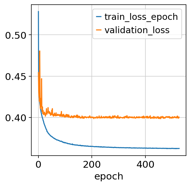
[18]:

fig, ax = plt.subplots()
bas.history_["train_loss_epoch"].plot(ax=ax)
bas.history_["validation_loss"].plot(ax=ax)

[18]:

<AxesSubplot: xlabel='epoch'>

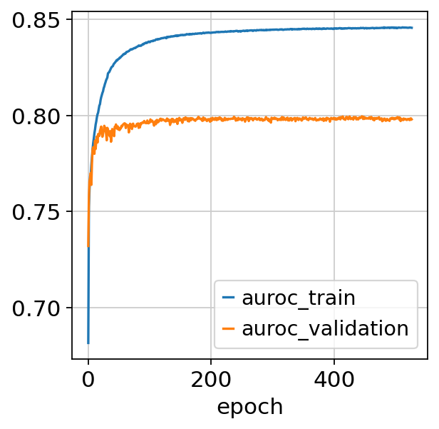
../../_images/tutorials_notebooks_scbasset_22_1.png

[19]:

fig, ax = plt.subplots()
bas.history_["auroc_train"].plot(ax=ax)
bas.history_["auroc_validation"].plot(ax=ax)

[19]:

<AxesSubplot: xlabel='epoch'>

../../_images/tutorials_notebooks_scbasset_23_1.png

Visualizing and analyzing the latent space#

We can now use the trained model to visualize, cluster, and analyze the data. We first extract the latent representation from the model, and save it back into our AnnData object:

[20]:

latent = bas.get_latent_representation()
adata.obsm["X_scbasset"] = latent

print(latent.shape)

(10970, 32)

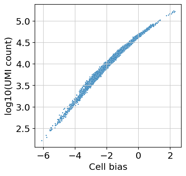
[21]:

sns.scatterplot(
    x=bas.get_cell_bias(),
    y=np.log10(np.asarray(adata.X.sum(1))).ravel(),
    s=3,
)
plt.xlabel("Cell bias")
plt.ylabel("log10(UMI count)")

[21]:

Text(0, 0.5, 'log10(UMI count)')

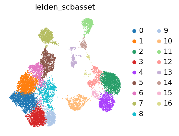
../../_images/tutorials_notebooks_scbasset_26_1.png

We can now use scanpy functions to cluster and visualize our latent space:

[23]:

# compute the k-nearest-neighbor graph that is used in both clustering and umap algorithms
sc.pp.neighbors(adata, use_rep="X_scbasset")
# compute the umap
sc.tl.umap(adata)
sc.tl.leiden(adata, key_added="leiden_scbasset")

[24]:

sc.pl.umap(adata, color="leiden_scbasset")

/home/adam/miniconda3/envs/scvi-tools-dev/lib/python3.10/site-packages/scanpy/plotting/_tools/scatterplots.py:392: UserWarning: No data for colormapping provided via 'c'. Parameters 'cmap' will be ignored
  cax = scatter(

../../_images/tutorials_notebooks_scbasset_29_1.png