Note
This page was generated from
totalvi_in_R.ipynb.
Interactive online version:
![]() .
Some tutorial content may look better in light mode.
.
Some tutorial content may look better in light mode.
CITE-seq analysis in R#
In this brief tutorial, we go over how to use scvi-tools functionality in R for analyzing CITE-seq data. We will closely follow the Bioconductor PBMC tutorial, using totalVI when appropriate.
This tutorial requires Reticulate. Please check out our installation guide for instructions on installing Reticulate and scvi-tools.
Loading and processing data with Bioconductor#
[3]:
library(BiocFileCache)
bfc <- BiocFileCache(ask=FALSE)
exprs.data <- bfcrpath(bfc, file.path(
    "http://cf.10xgenomics.com/samples/cell-vdj/3.1.0",
    "vdj_v1_hs_pbmc3",
    "vdj_v1_hs_pbmc3_filtered_feature_bc_matrix.tar.gz"))
untar(exprs.data, exdir=tempdir())

library(DropletUtils)
sce.pbmc <- read10xCounts(file.path(tempdir(), "filtered_feature_bc_matrix"))
sce.pbmc <- splitAltExps(sce.pbmc, rowData(sce.pbmc)$Type)
Loading required package: SingleCellExperiment

Loading required package: SummarizedExperiment

Loading required package: MatrixGenerics

Loading required package: matrixStats


Attaching package: ‘MatrixGenerics’


The following objects are masked from ‘package:matrixStats’:

    colAlls, colAnyNAs, colAnys, colAvgsPerRowSet, colCollapse,
    colCounts, colCummaxs, colCummins, colCumprods, colCumsums,
    colDiffs, colIQRDiffs, colIQRs, colLogSumExps, colMadDiffs,
    colMads, colMaxs, colMeans2, colMedians, colMins, colOrderStats,
    colProds, colQuantiles, colRanges, colRanks, colSdDiffs, colSds,
    colSums2, colTabulates, colVarDiffs, colVars, colWeightedMads,
    colWeightedMeans, colWeightedMedians, colWeightedSds,
    colWeightedVars, rowAlls, rowAnyNAs, rowAnys, rowAvgsPerColSet,
    rowCollapse, rowCounts, rowCummaxs, rowCummins, rowCumprods,
    rowCumsums, rowDiffs, rowIQRDiffs, rowIQRs, rowLogSumExps,
    rowMadDiffs, rowMads, rowMaxs, rowMeans2, rowMedians, rowMins,
    rowOrderStats, rowProds, rowQuantiles, rowRanges, rowRanks,
    rowSdDiffs, rowSds, rowSums2, rowTabulates, rowVarDiffs, rowVars,
    rowWeightedMads, rowWeightedMeans, rowWeightedMedians,
    rowWeightedSds, rowWeightedVars


Loading required package: GenomicRanges

Loading required package: stats4

Loading required package: BiocGenerics


Attaching package: ‘BiocGenerics’


The following objects are masked from ‘package:stats’:

    IQR, mad, sd, var, xtabs


The following objects are masked from ‘package:base’:

    anyDuplicated, append, as.data.frame, basename, cbind, colnames,
    dirname, do.call, duplicated, eval, evalq, Filter, Find, get, grep,
    grepl, intersect, is.unsorted, lapply, Map, mapply, match, mget,
    order, paste, pmax, pmax.int, pmin, pmin.int, Position, rank,
    rbind, Reduce, rownames, sapply, setdiff, sort, table, tapply,
    union, unique, unsplit, which.max, which.min


Loading required package: S4Vectors


Attaching package: ‘S4Vectors’


The following objects are masked from ‘package:base’:

    expand.grid, I, unname


Loading required package: IRanges

Loading required package: GenomeInfoDb

Loading required package: Biobase

Welcome to Bioconductor

    Vignettes contain introductory material; view with
    'browseVignettes()'. To cite Bioconductor, see
    'citation("Biobase")', and for packages 'citation("pkgname")'.


Attaching package: ‘Biobase’


The following object is masked from ‘package:MatrixGenerics’:

    rowMedians


The following objects are masked from ‘package:matrixStats’:

    anyMissing, rowMedians
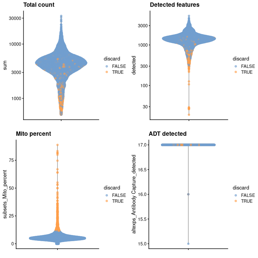
Pre-processing and quality control#
[4]:
unfiltered <- sce.pbmc
[5]:
library(scater)
is.mito <- grep("^MT-", rowData(sce.pbmc)$Symbol)
stats <- perCellQCMetrics(sce.pbmc, subsets=list(Mito=is.mito))

high.mito <- isOutlier(stats$subsets_Mito_percent, type="higher")
low.adt <- stats$`altexps_Antibody Capture_detected` < nrow(altExp(sce.pbmc))/2

discard <- high.mito | low.adt
sce.pbmc <- sce.pbmc[,!discard]
Loading required package: scuttle

Loading required package: ggplot2
[6]:
summary(high.mito)
   Mode   FALSE    TRUE
logical    6660     571
[7]:
colData(unfiltered) <- cbind(colData(unfiltered), stats)
unfiltered$discard <- discard

gridExtra::grid.arrange(
    plotColData(unfiltered, y="sum", colour_by="discard") +
        scale_y_log10() + ggtitle("Total count"),
    plotColData(unfiltered, y="detected", colour_by="discard") +
        scale_y_log10() + ggtitle("Detected features"),
    plotColData(unfiltered, y="subsets_Mito_percent",
        colour_by="discard") + ggtitle("Mito percent"),
    plotColData(unfiltered, y="altexps_Antibody Capture_detected",
        colour_by="discard") + ggtitle("ADT detected"),
    ncol=2
)
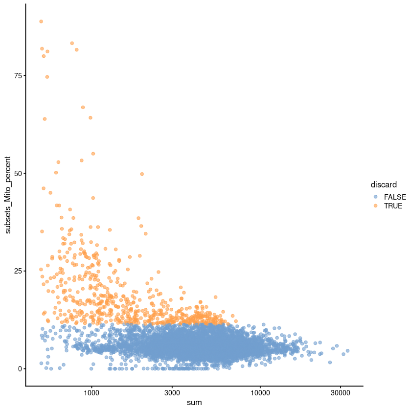
[8]:
plotColData(unfiltered, x="sum", y="subsets_Mito_percent",
    colour_by="discard") + scale_x_log10()
Normalization#
While we normalize the data here using standard Bioconductor practices, we will use the counts later for totalVI.
[11]:
library(scran)

set.seed(1000)
clusters <- quickCluster(sce.pbmc)
sce.pbmc <- computeSumFactors(sce.pbmc, cluster=clusters)
altExp(sce.pbmc) <- computeMedianFactors(altExp(sce.pbmc))
sce.pbmc <- logNormCounts(sce.pbmc, use_altexps=TRUE)
Warning message:
“'use.altexps=' is deprecated.
Use 'applySCE(x, logNormCounts)' instead.”
Data conversion (SCE -> AnnData)#
We use sceasy for conversion, and load the necessary Python packages for later.
[30]:
library(reticulate)
library(sceasy)
library(anndata)
use_python("/home/adam/.pyenv/versions/3.9.7/bin/python", required = TRUE)
sc <- import("scanpy", convert = FALSE)
scvi <- import("scvi", convert = FALSE)
sys <- import ("sys", convert = FALSE)
We make two AnnData objects, one per modality, and then store the protein counts in the canonical location for scvi-tools.
[24]:
adata <- convertFormat(sce.pbmc, from="sce", to="anndata", main_layer="counts", drop_single_values=FALSE)
adata_protein <- convertFormat(altExp(sce.pbmc), from="sce", to="anndata", main_layer="counts", drop_single_values=FALSE)
adata$obsm["protein"] <- adata_protein$to_df()
[28]:
adata
AnnData object with n_obs × n_vars = 6660 × 33538
    obs: 'Sample', 'Barcode', 'sizeFactor'
    var: 'ID', 'Symbol', 'Type'
    obsm: 'protein'
Run totalVI for dimensionality reduction#
totalVI will output a low-dimensional representation of cells that captures information from both the RNA and protein. Here we show how to use totalVI for only dimensionality reduction, though totalVI can perform other tasks that are shown in the Python-based tutorials. The intention here is to provide some examples of how to use totalVI from R.
[31]:
scvi$model$TOTALVI$setup_anndata(adata, protein_expression_obsm_key="protein")
None
None
[32]:
vae <- scvi$model$TOTALVI(adata)
vae$train()
None
[38]:
reducedDims(sce.pbmc) <- list(TOTALVI=py_to_r(vae$get_latent_representation()))
sce.pbmc <- runUMAP(sce.pbmc, dimred="TOTALVI")
sce.pbmc <- runTSNE(sce.pbmc, dimred="TOTALVI")
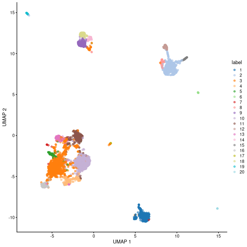
Clustering#
[39]:
g <- buildSNNGraph(sce.pbmc, k=10, use.dimred = 'TOTALVI')
clust <- igraph::cluster_walktrap(g)$membership
colLabels(sce.pbmc) <- factor(clust)
[37]:
plotUMAP(sce.pbmc, colour_by="label")
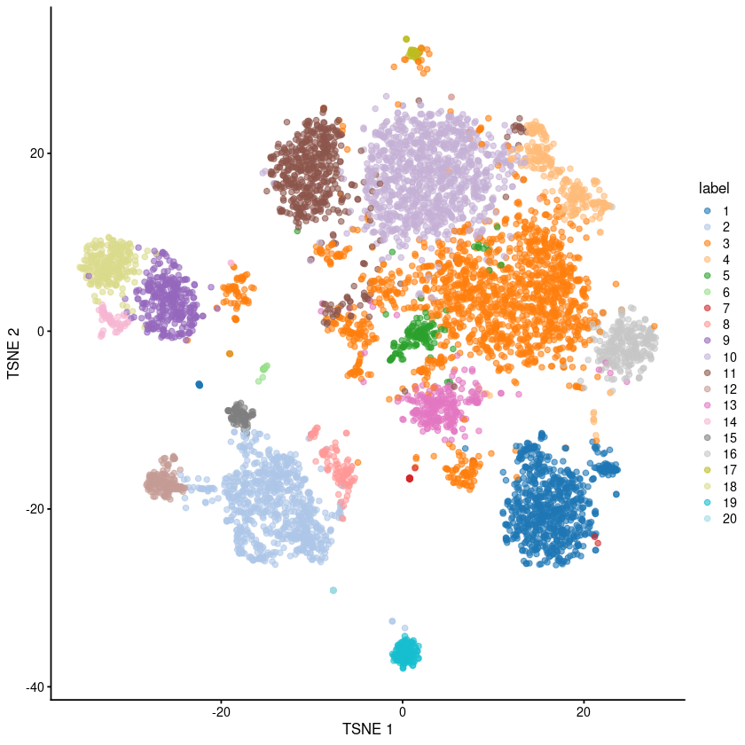
[40]:
plotTSNE(sce.pbmc, colour_by="label")
[43]:
sI <- sessionInfo()
sI$loadedOnly <- NULL
print(sI, locale=FALSE)
R version 4.1.0 (2021-05-18)
Platform: x86_64-pc-linux-gnu (64-bit)
Running under: Ubuntu 20.04.2 LTS

Matrix products: default
BLAS:   /usr/lib/x86_64-linux-gnu/blas/libblas.so.3.9.0
LAPACK: /usr/lib/x86_64-linux-gnu/lapack/liblapack.so.3.9.0

attached base packages:
[1] stats4    stats     graphics  grDevices utils     datasets  methods
[8] base

other attached packages:
 [1] anndata_0.7.5.3             sceasy_0.0.6
 [3] reticulate_1.20             scran_1.21.3
 [5] scater_1.21.3               ggplot2_3.3.5
 [7] scuttle_1.3.1               DropletUtils_1.13.2
 [9] SingleCellExperiment_1.15.2 SummarizedExperiment_1.23.4
[11] Biobase_2.53.0              GenomicRanges_1.45.0
[13] GenomeInfoDb_1.29.8         IRanges_2.27.2
[15] S4Vectors_0.31.3            BiocGenerics_0.39.2
[17] MatrixGenerics_1.5.4        matrixStats_0.60.1
[19] BiocFileCache_2.1.1         dbplyr_2.1.1