VIVS: identifying genes that depend on the cellular niche

VIVS: identifying genes that depend on the cellular niche#

This tutorial demonstrates VIVS [Boyeau et al., 2024], a conditional randomization test (CRT) that identifies which genes in a cell’s expression profile are conditionally dependent on an external response of interest. VIVS learns (or reuses) a deep generative model of gene expression as a calibrated “knockoff” sampler, then tests whether an importance-score network can predict the response Y from the true expression better than from knockoff draws, yielding FDR-controlled p-values per gene (and, via a hierarchical extension, per gene cluster at several resolutions).

Here, Y is a niche-composition vector we compute directly from spatial coordinates (the cell-type composition of each cell’s spatial neighborhood), and the knockoff sampler is a plain SCVI model trained on the raw counts — VIVS works with any generative model whose module is a scvi.module.VAE subclass (see VIVS for the full compatibility table), not just spatially-aware ones.

import os
import tempfile

import numpy as np
import pandas as pd
import scanpy as sc
import scvi
from scvi.external import VIVS
from scvi.external.vivs import plot_hier_importance
from sklearn.neighbors import NearestNeighbors

scvi.settings.seed = 0
print("Last run with scvi-tools version:", scvi.__version__)

Last run with scvi-tools version: 1.5.0.post1

Data loading#

In this tutorial we load a human breast cancer section, generated with 10X Xenium. The cell segmentation originally performed on this data resulted in many erroneously assigned transcripts and therefore re-segmented the cells using the ProSeg algorithm, which is a scalable algorithm for transcriptome-informed segmentation.

save_dir = tempfile.TemporaryDirectory()

adata_path = os.path.join(save_dir.name, "adata_for_tuto_s1.h5ad")
adata = sc.read(
    adata_path,
    backup_url="https://exampledata.scverse.org/scvi-tools/adata_for_tuto_s1.h5ad",
)
adata

AnnData object with n_obs × n_vars = 117305 × 313
    obs: 'sample', 'x', 'y', 'z', 'observed_x', 'observed_y', 'observed_z', 'fov', 'n_counts', 'index', 'cell_type'
    var: 'mt'
    uns: '_scvi_manager_uuid', '_scvi_uuid', 'log1p', 'pca'
    obsm: 'X_pca', 'X_scANVI', 'spatial'
    varm: 'PCs'
    layers: 'counts', 'counts_log1p', 'counts_wo_bg', 'min_max_scaled', 'min_max_scaled_raw', None (.X)

Compute the niche composition#

VIVS needs a response Y to test gene expression against — here, for every cell, the cell-type composition of its k-nearest spatial neighbors (\(k=20\)), restricted to neighbors on the same slide (sample), since spatial coordinates aren’t comparable across independent sections. This is a plain k-NN + one-hot-average computation, with no dependency on any particular generative model.

def compute_niche_composition(
    adata,
    k_nn: int = 20,
    sample_key: str = "sample",
    labels_key: str = "cell_type",
    cell_coordinates_key: str = "spatial",
    niche_composition_key: str = "niche_composition",
) -> None:
    """Compute, for every cell, the cell-type composition of its k-nearest spatial neighbors."""
    cell_types = adata.obs[labels_key].astype("category")
    one_hot = pd.get_dummies(cell_types).values.astype(np.float32)
    niche_composition = np.zeros((adata.n_obs, one_hot.shape[1]), dtype=np.float32)

    for sample in adata.obs[sample_key].unique():
        mask = (adata.obs[sample_key] == sample).values
        coords = adata.obsm[cell_coordinates_key][mask]
        n_neighbors = min(k_nn + 1, mask.sum())
        _, indices = NearestNeighbors(n_neighbors=n_neighbors).fit(coords).kneighbors(coords)
        # indices[:, 0] is always the cell itself; average over the remaining neighbors
        niche_composition[mask] = one_hot[mask][indices[:, 1:]].mean(axis=1)

    adata.obsm[niche_composition_key] = niche_composition


compute_niche_composition(adata, k_nn=20)

Train a plain SCVI model#

We register the adata and train a plain SCVI model to convergence. Its trained module will be reused below as VIVS’s knockoff sampler, so VIVS itself will skip fitting its own generative VAE (phase 1) and go directly to testing niche_composition dependence (phase 2).

scvi.model.SCVI.setup_anndata(
    adata,
    layer="counts",  # adata layer that contains the raw counts
    batch_key="sample",  # column in adata.obs that contains the batch covariate
)

scvi_model = scvi.model.SCVI(adata)
scvi_model.train(
    max_epochs=200,
    early_stopping=True,
    check_val_every_n_epoch=1,
    batch_size=512,
    plan_kwargs={
        "lr": 5e-4,
    },
)

Test niche-composition dependence with VIVS#

We register the same adata for VIVS, with y_obsm_key="niche_composition" as the response Y whose dependence on gene expression X we want to test. Passing x_model=scvi_model tells VIVS to reuse the already-trained SCVI module (frozen) as its knockoff sampler, instead of fitting a new generative VAE — VIVS’s .train() call then only fits the importance-score network for Y | X.

VIVS.setup_anndata(
    adata,
    y_obsm_key="niche_composition",  # cell-type composition of each cell's spatial neighborhood
    layer="counts",  # same raw-count layer used to train SCVI
    batch_key="sample",  # column in adata.obs that contains the batch covariate
)

vivs_model = VIVS(adata, x_model=scvi_model)
vivs_model.train(max_epochs=200)

INFO     Generating sequential column names

Visualizing results#

plot_hier_importance renders the multi-resolution results as a significance dendrogram: genes/clusters found significant (BH-adjusted p-value below significance_threshold) at the coarsest resolution are shown, colored by significance, across all tested resolutions.

plot_hier_importance(res, theme_kwargs={"figure_size": (15, 3)})

../../../_images/7b3ac16d5627c007049a6a89e80e07f01ce0419435e0df90a1e09b8a58b35776.png

# p-values on the held-out validation split (the default -- see `get_importance`'s docstring)
vivs_model_res = vivs_model.get_importance(indices=vivs_model.validation_indices, n_mc_samples=200)
pvalues = vivs_model_res["pvalues"][:, 0]

INFO     Generating sequential column names

import matplotlib.pyplot as plt

fig, ax = plt.subplots(figsize=(5, 4))
ax.hist(pvalues, bins=20, range=(0, 1), density=True, alpha=0.8)
ax.axhline(1.0, color="black", linestyle="--", linewidth=1)
ax.set_xlabel("p-value")
ax.set_ylabel("density")
ax.set_title("VIVS model: p-value histogram")
ax.legend()
fig.tight_layout()
fig

../../../_images/e8ae5535d5f216631c48533276f13d60f031553e0180c6c365f9e306284ddbe0.png

Interpretation and next steps#

A gene (or gene cluster) called significant at a given resolution means the CRT rejected the null hypothesis that gene expression is conditionally independent of the niche composition Y, at the chosen FDR level, when knockoffs are drawn from SCVI’s generative model — i.e. that gene’s expression carries information about the surrounding niche beyond what is already explained by every other gene. Coarser resolutions (larger gene clusters) aggregate evidence across correlated genes and tend to have more power to detect weaker, distributed niche effects, while the finest (per-gene) resolution pinpoints individual genes.

For a per-cell rather than per-dataset view of which cells drive a given gene’s (or gene cluster’s) importance score, see get_cell_scores(), which returns unsummed, per-cell importance scores for a chosen set of genes and responses.

Sanity check: is VIVS calibrated on this data?#

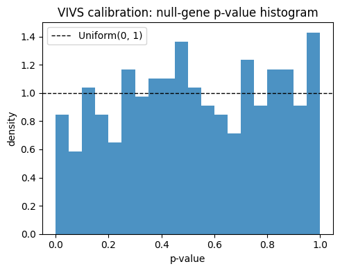
Ground truth is unknown for niche_composition on real data, so the significant genes found above cannot be directly checked against a known answer. To still validate that VIVS’s p-values are calibrated on this dataset (same cell count, same expression noise, same batch structure), we build a semi-synthetic response: a nonlinear function of a handful of “true” genes’ own expression, plus Gaussian noise. Genes not among these “true” genes are, by construction, conditionally independent of the response given the rest of the transcriptome — so under a well-calibrated CRT, their p-values (computed on the held-out validation split) should look ~Uniform(0, 1), while the true genes’ p-values should be very small.

This reuses the already-trained scvi_model as the knockoff sampler (as above), so only a new importance-score net needs to be fit.

N_TRUE_GENES = 5
rng = np.random.default_rng(0)

true_gene_idx = rng.choice(adata.n_vars, size=N_TRUE_GENES, replace=False)
x_true = adata.layers["counts_log1p"][:, true_gene_idx]
if hasattr(x_true, "todense"):
    x_true = np.asarray(x_true.todense())
x_true = x_true - x_true.mean(0, keepdims=True)

# nonlinear (quadratic) combination of the true genes, corrupted by Gaussian noise
y_synthetic = (x_true**2).sum(1, keepdims=True)
y_synthetic = y_synthetic + rng.normal(scale=y_synthetic.std() * 0.5, size=y_synthetic.shape)
adata.obsm["synthetic_niche"] = y_synthetic.astype(np.float32)

print("true genes:", adata.var_names[true_gene_idx].tolist())

true genes: ['MPO', 'KIT', 'CTSG', 'DNAAF1', 'SLAMF1']

VIVS.setup_anndata(
    adata,
    y_obsm_key="synthetic_niche",
    layer="counts",
    batch_key="sample",
)

calibration_model = VIVS(adata, x_model=scvi_model)
calibration_model.train(max_epochs=200)

INFO     Generating sequential column names

# p-values on the held-out validation split (the default -- see `get_importance`'s docstring)
calib_res = calibration_model.get_importance(
    indices=calibration_model.validation_indices, n_mc_samples=200
)
pvalues = calib_res["pvalues"][:, 0]

is_true_gene = np.isin(np.arange(adata.n_vars), true_gene_idx)
null_pvalues = pvalues[~is_true_gene]
print(f"null p-values: mean={null_pvalues.mean():.3f} (should be close to 0.5 if calibrated)")
print("true-gene p-values:", pvalues[is_true_gene])

null p-values: mean=0.528 (should be close to 0.5 if calibrated)
true-gene p-values: [0.00497512 0.00497512 0.00497512 0.00497512 0.00497512]

import matplotlib.pyplot as plt

fig, ax = plt.subplots(figsize=(5, 4))
ax.hist(null_pvalues, bins=20, range=(0, 1), density=True, alpha=0.8)
ax.axhline(1.0, color="black", linestyle="--", linewidth=1, label="Uniform(0, 1)")
ax.set_xlabel("p-value")
ax.set_ylabel("density")
ax.set_title("VIVS calibration: null-gene p-value histogram")
ax.legend()
fig.tight_layout()
fig

../../../_images/13e0b460080654dcdd867caf62bc2d5634ec59582fa7cbe533215eef7ba9b5b6.png