Differential expression on Packer C. elegans data
This notebook was contributed by Eduardo Beltrame [@Munfred](https://github.com/Munfred) and edited by Romain Lopez with help from Adam Gayoso.
Processing and visualizing 89k cells from Packer et al. 2019 C. elegans 10xv2 single cell data
Original article: A lineage-resolved molecular atlas of C. elegans embryogenesis at single-cell resolution
https://science.sciencemag.org/content/365/6459/eaax1971.long
The anndata object we provide has 89701 cells and 20222 genes. It includes short gene descriptions from WormBase that will show up when mousing over the interactive plots.
Steps performed:
Loading the data from anndata containing cell labels and gene descriptions
Training the model with batch labels for integration with scVI
Retrieving the scVI latent space and imputed values
Visualize the latent space with an interactive UMAP plot using Plotly
Perform differential expression and visualize with interactive volcano plot and heatmap using Plotly
This notebook was designed to be run in Google Colab.
![]()
[ ]:
# If running in Colab, navigate to Runtime -> Change runtime type
# and ensure you're using a Python 3 runtime with GPU hardware accelerator
# Installation of scVI in Colab can take several minutes
[ ]:
import sys
IN_COLAB = "google.colab" in sys.modules
show_plot = True
save_path = "./"
if IN_COLAB:
!pip install --quiet scvi[notebooks]==0.6.3
[4]:
import scvi
scvi.__version__
[4]:
'0.6.3'
[ ]:
%matplotlib inline
%config InlineBackend.figure_format = 'retina'
# Control warnings
import warnings; warnings.simplefilter('ignore')
import os
import numpy as np
import pandas as pd
import matplotlib.pyplot as plt
from scvi.dataset import GeneExpressionDataset
from scvi.models import VAE
from scvi.inference import UnsupervisedTrainer
import torch
import anndata
import plotly.express as px
import plotly.graph_objects as go
from umap import UMAP
if IN_COLAB:
%matplotlib inline
[6]:
## Change the path where the models will be saved
save_path = "./"
vae_file_name = 'worm_vae.pkl'
if os.path.isfile('packer2019.h5ad'):
print ("Found the data file! No need to download.")
else:
print ("Downloading data...")
! wget https://github.com/Munfred/wormcells-site/releases/download/packer2019/packer2019.h5ad
Found the data file! No need to download.
[ ]:
adata = anndata.read('packer2019.h5ad')
[8]:
adata
[8]:
AnnData object with n_obs × n_vars = 89701 × 20222
obs: 'cell', 'numi', 'time_point', 'batch', 'size_factor', 'cell_type', 'cell_subtype', 'plot_cell_type', 'raw_embryo_time', 'embryo_time', 'embryo_time_bin', 'raw_embryo_time_bin', 'lineage', 'passed_qc'
var: 'gene_id', 'gene_name', 'gene_description'
[9]:
adata.X
[9]:
<89701x20222 sparse matrix of type '<class 'numpy.float32'>'
with 82802059 stored elements in Compressed Sparse Column format>
Take a look at the gene descriptions
The gene descriptions were taken using the WormBase API.
[10]:
display(adata.var.head().style.set_properties(subset=['gene_description'], **{'width': '600px'}))
| gene_id | gene_name | gene_description | |
|---|---|---|---|
| index | |||
| WBGene00010957 | WBGene00010957 | nduo-6 | Is affected by several genes including daf-16; daf-12; and hsf-1 based on RNA-seq and tiling array studies. Is affected by six chemicals including Rotenone; Psoralens; and metformin based on RNA-seq and microarray studies. |
| WBGene00010958 | WBGene00010958 | ndfl-4 | Is enriched in Psub2 based on RNA-seq studies. Is affected by several genes including daf-16; daf-12; and clk-1 based on RNA-seq and microarray studies. Is affected by six chemicals including Alovudine; Psoralens; and metformin based on RNA-seq studies. |
| WBGene00010959 | WBGene00010959 | nduo-1 | Is an ortholog of human MT-ND1 (mitochondrially encoded NADH:ubiquinone oxidoreductase core subunit 1). Is predicted to contribute to NADH dehydrogenase activity. Human ortholog(s) of this gene are implicated in Leber hereditary optic neuropathy and MELAS syndrome. |
| WBGene00010960 | WBGene00010960 | atp-6 | Is predicted to contribute to proton-transporting ATP synthase activity, rotational mechanism. |
| WBGene00010961 | WBGene00010961 | nduo-2 | Is affected by several genes including hsf-1; clk-1; and elt-2 based on RNA-seq and microarray studies. Is affected by eight chemicals including stavudine; Zidovudine; and Psoralens based on RNA-seq and microarray studies. |
[11]:
adata.obs.head().T
[11]:
| index | AAACCTGAGACAATAC-300.1.1 | AAACCTGAGGGCTCTC-300.1.1 | AAACCTGAGTGCGTGA-300.1.1 | AAACCTGAGTTGAGTA-300.1.1 | AAACCTGCAAGACGTG-300.1.1 |
|---|---|---|---|---|---|
| cell | AAACCTGAGACAATAC-300.1.1 | AAACCTGAGGGCTCTC-300.1.1 | AAACCTGAGTGCGTGA-300.1.1 | AAACCTGAGTTGAGTA-300.1.1 | AAACCTGCAAGACGTG-300.1.1 |
| numi | 1630 | 2319 | 3719 | 4251 | 1003 |
| time_point | 300_minutes | 300_minutes | 300_minutes | 300_minutes | 300_minutes |
| batch | Waterston_300_minutes | Waterston_300_minutes | Waterston_300_minutes | Waterston_300_minutes | Waterston_300_minutes |
| size_factor | 1.02319 | 1.45821 | 2.33828 | 2.65905 | 0.62961 |
| cell_type | Body_wall_muscle | nan | nan | Body_wall_muscle | Ciliated_amphid_neuron |
| cell_subtype | BWM_head_row_1 | nan | nan | BWM_anterior | AFD |
| plot_cell_type | BWM_head_row_1 | nan | nan | BWM_anterior | AFD |
| raw_embryo_time | 360 | 260 | 270 | 260 | 350 |
| embryo_time | 380 | 220 | 230 | 280 | 350 |
| embryo_time_bin | 330-390 | 210-270 | 210-270 | 270-330 | 330-390 |
| raw_embryo_time_bin | 330-390 | 210-270 | 270-330 | 210-270 | 330-390 |
| lineage | MSxpappp | MSxapaap | nan | Dxap | ABalpppapav/ABpraaaapav |
| passed_qc | True | True | True | True | True |
Loading data
We load the Packer data and use the batch annotations for scVI. Here, each experiment correspond to a batch.
[12]:
gene_dataset = GeneExpressionDataset()
# we provide the `batch_indices` so that scvi can perform batch correction
gene_dataset.populate_from_data(
adata.X,
gene_names=adata.var.index.values,
cell_types=adata.obs['cell_type'].values,
batch_indices=adata.obs['batch'].cat.codes.values,
)
# We select the 1000 most variable genes, which is a recommended selection criteria of scvi
# this method in particular is based on the method of Seurat v3
gene_dataset.subsample_genes(1000)
sel_genes = gene_dataset.gene_names
[2020-04-02 03:49:05,753] INFO - scvi.dataset.dataset | Remapping labels to [0,N]
[2020-04-02 03:49:05,759] INFO - scvi.dataset.dataset | Remapping batch_indices to [0,N]
[2020-04-02 03:49:05,765] INFO - scvi.dataset.dataset | extracting highly variable genes using seurat_v3 flavor
Transforming to str index.
[2020-04-02 03:49:56,429] INFO - scvi.dataset.dataset | Downsampling from 20222 to 1000 genes
[2020-04-02 03:49:56,775] INFO - scvi.dataset.dataset | Computing the library size for the new data
[2020-04-02 03:49:57,163] INFO - scvi.dataset.dataset | Filtering non-expressing cells.
[2020-04-02 03:49:57,579] INFO - scvi.dataset.dataset | Computing the library size for the new data
[2020-04-02 03:49:57,965] INFO - scvi.dataset.dataset | Downsampled from 89701 to 89701 cells
At this point we may make the scVI dataset RNA count matrix dense, as we filtered the genes. This makes inference faster because when the matrix is sparse, the trainer has to make each minibatch dense before it loads it on the model and the GPU is using CUDA.
[13]:
gene_dataset.X = gene_dataset.X.toarray()
[2020-04-02 03:50:00,523] INFO - scvi.dataset.dataset | Computing the library size for the new data
[14]:
adata.obs['cell_type'].values
[14]:
[Body_wall_muscle, nan, nan, Body_wall_muscle, Ciliated_amphid_neuron, ..., Rectal_gland, nan, nan, nan, nan]
Length: 89701
Categories (37, object): [ABarpaaa_lineage, Arcade_cell, Body_wall_muscle, Ciliated_amphid_neuron, ...,
hmc_and_homolog, hmc_homolog, hyp1V_and_ant_arc_V, nan]
Training
n_epochs: Maximum number of epochs to train the model. If the likelihood change is small than a set threshold training will stop automatically.
lr: learning rate. Set to 0.001 here.
use_cuda: Set to true to use CUDA (GPU required)
[ ]:
# for this dataset 50 epochs is sufficient
# note that smaller datasets require hundreds of epochs
n_epochs = 50
lr = 1e-3
use_cuda = True
We now create the model and the trainer object. We train the model and output model likelihood every epoch. In order to evaluate the likelihood on a test set, we split the datasets (the current code can also so train/validation/test).
If a pre-trained model already exist in the save_path then load the same model rather than re-training it. This is particularly useful for large datasets.
[ ]:
# set the VAE to perform batch correction
vae = VAE(gene_dataset.nb_genes, n_batch=gene_dataset.n_batches)
[ ]:
# Use per minibatch warmup (iters) for large datasets
trainer = UnsupervisedTrainer(
vae,
gene_dataset,
train_size=0.85, # number between 0 and 1, default 0.8
use_cuda=use_cuda,
frequency=1,
n_epochs_kl_warmup=None,
n_iter_kl_warmup=int(128*5000/400)
)
[18]:
# check if a previously trained model already exists, if yes load it
full_file_save_path = os.path.join(save_path, vae_file_name)
if os.path.isfile(full_file_save_path):
trainer.model.load_state_dict(torch.load(full_file_save_path))
trainer.model.eval()
else:
trainer.train(n_epochs=n_epochs, lr=lr)
torch.save(trainer.model.state_dict(), full_file_save_path)
[2020-04-02 03:50:07,270] INFO - scvi.inference.inference | KL warmup for 1600 iterations
training: 100%|██████████| 50/50 [08:53<00:00, 10.66s/it]
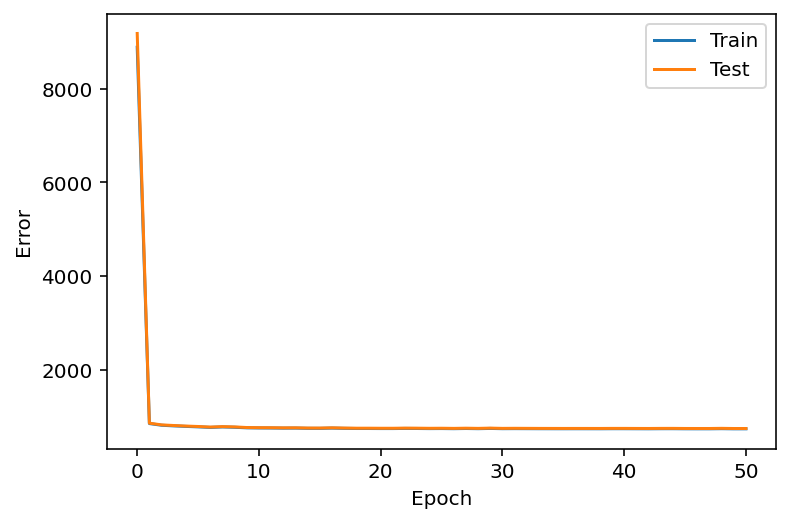
Plotting the likelihood change across training
[19]:
train_test_results = pd.DataFrame(trainer.history).rename(columns={'elbo_train_set':'Train', 'elbo_test_set':'Test'})
train_test_results
[19]:
| Train | Test | |
|---|---|---|
| 0 | 8881.413828 | 9174.447856 |
| 1 | 857.742913 | 865.714189 |
| 2 | 821.685303 | 829.391246 |
| 3 | 808.042363 | 816.110580 |
| 4 | 796.994002 | 804.426280 |
| 5 | 787.069519 | 795.110373 |
| 6 | 775.612372 | 782.976124 |
| 7 | 785.185200 | 792.350435 |
| 8 | 778.276230 | 786.173274 |
| 9 | 766.440439 | 773.111641 |
| 10 | 763.470819 | 770.053581 |
| 11 | 762.309879 | 769.090608 |
| 12 | 759.699914 | 766.290829 |
| 13 | 760.565406 | 767.061953 |
| 14 | 755.770818 | 762.247230 |
| 15 | 755.289439 | 761.668258 |
| 16 | 760.560715 | 767.147357 |
| 17 | 755.285547 | 761.907396 |
| 18 | 752.282227 | 758.606450 |
| 19 | 752.231292 | 758.707572 |
| 20 | 751.001023 | 757.318010 |
| 21 | 750.882924 | 757.270630 |
| 22 | 753.712712 | 760.248563 |
| 23 | 752.402924 | 759.038684 |
| 24 | 750.010072 | 756.424613 |
| 25 | 751.233984 | 757.741389 |
| 26 | 748.450227 | 754.827124 |
| 27 | 752.164061 | 758.740302 |
| 28 | 748.442852 | 754.916773 |
| 29 | 753.610544 | 760.393845 |
| 30 | 748.497168 | 755.029036 |
| 31 | 749.499188 | 756.388857 |
| 32 | 748.662938 | 755.379153 |
| 33 | 747.743216 | 754.304865 |
| 34 | 747.289906 | 753.938626 |
| 35 | 746.901389 | 753.527914 |
| 36 | 747.174424 | 753.747798 |
| 37 | 746.882975 | 753.544082 |
| 38 | 746.582319 | 753.286055 |
| 39 | 747.826352 | 754.543043 |
| 40 | 747.763953 | 754.599980 |
| 41 | 746.903656 | 753.518663 |
| 42 | 746.093606 | 752.914513 |
| 43 | 747.682025 | 754.577081 |
| 44 | 748.042126 | 754.908751 |
| 45 | 746.043148 | 752.920929 |
| 46 | 745.559933 | 752.408477 |
| 47 | 745.672933 | 752.533768 |
| 48 | 748.517461 | 755.667539 |
| 49 | 745.237304 | 752.205676 |
| 50 | 745.312490 | 752.293802 |
[20]:
ax = train_test_results.plot()
ax.set_xlabel("Epoch")
ax.set_ylabel("Error")
plt.show()
Obtaining the posterior object and sample latent space
The posterior object contains a model and a gene_dataset, as well as additional arguments that for Pytorch’s DataLoader. It also comes with many methods or utilities querying the model, such as differential expression, imputation and differential analyisis.
To get an ordered output result, we might use .sequential posterior’s method which return another instance of posterior (with shallow copy of all its object references), but where the iteration is in the same ordered as its indices attribute.
[21]:
# This provides a posterior with sequential index sampling
full = trainer.create_posterior()
latent, batch_indices, labels = full.get_latent()
batch_indices = batch_indices.ravel()
latent.shape
[21]:
(89701, 10)
[22]:
# store the latent space in a new anndata object
post_adata = anndata.AnnData(X=gene_dataset.X)
post_adata.obs=adata.obs
post_adata.obsm["latent"] = latent
post_adata
[22]:
AnnData object with n_obs × n_vars = 89701 × 1000
obs: 'cell', 'numi', 'time_point', 'batch', 'size_factor', 'cell_type', 'cell_subtype', 'plot_cell_type', 'raw_embryo_time', 'embryo_time', 'embryo_time_bin', 'raw_embryo_time_bin', 'lineage', 'passed_qc'
obsm: 'latent'
Using Plotly’s Scattergl we can easily and speedily make interactive plots with 89k cells!
[ ]:
# here's a hack to randomize categorical colors, since plotly can't do that in a straightforward manner
# we take the list of named css colors that it recognizes, and we picked a color based on the code of
# the cluster we are coloring
css_colors=[
'aliceblue','antiquewhite','aqua','aquamarine','azure','bisque','black','blanchedalmond','blue',
'blueviolet','brown','burlywood','cadetblue','chartreuse','chocolate','coral','cornflowerblue',
'crimson','cyan','darkblue','darkcyan','darkgoldenrod','darkgray','darkgrey','darkgreen','darkkhaki',
'darkmagenta','darkolivegreen','darkorange','darkorchid','darkred','darksalmon','darkseagreen',
'darkslateblue','darkslategray','darkslategrey','darkturquoise','darkviolet','deeppink','deepskyblue',
'dimgray','dimgrey','dodgerblue','firebrick','floralwhite','forestgreen','fuchsia','gainsboro','ghostwhite',
'gold','goldenrod','gray','grey','green','greenyellow','honeydew','hotpink','indianred','indigo',
'ivory','khaki','lavender','lavenderblush','lawngreen','lemonchiffon','lightblue','lightcoral','lightcyan',
'lightgoldenrodyellow','lightgray','lightgrey','lightgreen','lightpink','lightsalmon','lightseagreen',
'lightskyblue','lightslategray','lightslategrey','lightsteelblue','lightyellow','lime','limegreen','linen',
'magenta','maroon','mediumaquamarine','mediumblue','mediumorchid','mediumpurple','mediumseagreen',
'mediumslateblue','mediumspringgreen','mediumturquoise','mediumvioletred','midnightblue','mintcream',
'mistyrose','moccasin','navajowhite','navy','oldlace','olive','olivedrab','orange','orangered','orchid',
'palegoldenrod','palegreen','paleturquoise','palevioletred','papayawhip','peachpuff','peru','pink','plum'
,'powderblue','purple','red','rosybrown','royalblue','saddlebrown','salmon','sandybrown','seagreen',
'seashell','sienna','silver','skyblue','slateblue','slategray','slategrey','snow','springgreen','steelblue',
'tan','teal','thistle','tomato','turquoise','violet','wheat','white','whitesmoke','yellow','yellowgreen']
# we just repeat the list of colors a bunch of times to ensure we always have more colors than clusters
css_colors = css_colors*100
# now define a function to plot any embedding
def plot_embedding(embedding_kind, # the embedding must be a label in the post_adata.obsm
adata=adata, # the original adata for taking the cluster labels
post_adata=post_adata,
cluster_feature ='cell_type',
xlabel="Dimension 1",
ylabel="Dimension 2",
plot_title="Embedding on single cell data"):
# `cluster_feature` should be the name of one of the categorical annotation columns
# e.g. `cell_type`, `cell_subtype`, `time_point`
cluster_ids = adata.obs[cluster_feature].cat.codes.unique()
id_to_cluster_map = dict( zip( adata.obs[cluster_feature].cat.codes, adata.obs[cluster_feature] ) )
cluster_to_id_map = dict([[v,k] for k,v in id_to_cluster_map.items()])
fig = go.Figure()
for _cluster_id in adata.obs[cluster_feature].cat.codes.unique():
fig.add_trace(
go.Scattergl(
x = post_adata.obsm[embedding_kind][:,0][post_adata.obs[cluster_feature].cat.codes==_cluster_id]
, y = post_adata.obsm[embedding_kind][:,1][post_adata.obs[cluster_feature].cat.codes==_cluster_id]
, mode='markers'
, marker=dict(
# we randomize colors by starting at a random place in the list of named css colors
color=css_colors[_cluster_id+np.random.randint(0,len(np.unique(css_colors)))]
, size = 3
)
, showlegend=True
, name=id_to_cluster_map[_cluster_id]
, hoverinfo=['name']
)
)
layout={
"title": {"text": plot_title
, 'x':0.5
}
, 'xaxis': {'title': {"text": xlabel}}
, 'yaxis': {'title': {"text": ylabel}}
, "height": 800
, "width":1000
}
fig.update_layout(layout)
fig.update_layout(showlegend=True)
return fig
[ ]:
latent_umap = UMAP(spread=2).fit_transform(latent)
[ ]:
post_adata.obsm["UMAP"] = np.array(latent_umap)
[ ]:
fig = plot_embedding(embedding_kind='UMAP',
cluster_feature ='cell_type',
xlabel="UMAP 1",
ylabel="UMAP 2",
plot_title="UMAP on scVI latent space for Packer C. elegans single cell data")
[27]:
# uncomment this line to save an interactive html plot, in case it is not rendering
#fig.write_html('worms_interactive_tsne.html')
fig.show()
Performing Differential Expression with vanilla and change modes
Note: scVI recently introduced a second way to perform DE, and some functions and documentation are still changing. The old mode is called ``vanilla`` and is performed below. The new mode is called ``change`` and is done at the end of the notebook. In addition to Bayes Factors, the new ``change`` mode allows for calculating p-values, which are more commonly seen in volcano plots.
From the trained VAE model we can sample the gene expression rate for each gene in each cell.
For two populations of interest, we can then randomly sample pairs of cells, one from each population to compare their expression rate for a gene.
In the
vanillamode, DE is measured by logit(p/(1-p)) where p is the probability of a cell from population A having a higher expression than a cell from population B.We can form the null distribution of the DE values by sampling pairs randomly from the combined population.
Explanation of Vanilla DE mode and Bayes Factors
Explanation adapted from the scVi `differential_expression_score docstring <https://github.com/YosefLab/scVI/blob/05920d1f85daa362d4fb694e588ab090bc84e207/scvi/inference/posterior.py#L640>`__.
The ``vanilla`` mode follows protocol described in Lopez et al, arXiv:1709.02082.
In this case for a given gene we perform hypothesis testing based on latent variable in the generative model that models the mean of the gene expression.
We are comparing \(h_{1g}\), the mean expression of gene \(g\) in cell type 1, with \(h_{2g}\), the mean expression of \(g\) in cell type 2.
The hypotheses are:
DE between cell types 1 and 2 for each gene can then be based on the Bayes factors:
Note that the scvi ``differential_expression_score`` returns the *natural logarithm* of the Bayes Factor. This is :math:`ln(BF_{10})` in the table discussed below.
To compute the gene specific Bayes factors using masks idx1 and idx2 we sample the Posterior in the following way:
The posterior is sampled
n_samplestimes for each subpopulationFor computation efficiency (posterior sampling is quite expensive), instead of comparing element-wise the obtained samples, we can permute posterior samples.
Remember that computing the Bayes Factor requires sampling \(q(z_A | x_A)\) and \(q(z_B | x_B)\)
Interpreting Bayes factors
To learn more about Bayes factors vs. p-values, see the review On p-Values and Bayes Factors by Leonhard Held and Manuela Ott.
Bayes factor \(BF_{10}\) |
\(\ln(BF_{10})\) |
Interpretation |
|---|---|---|
> 100 |
> 4.60 |
Extreme evidence for H1 |
30 – 100 |
(3.4, 4.6) |
Very strong evidence for H1 |
10 – 30 |
(2.3, 3.4) |
Strong evidence for H1 |
3 – 10 |
(1.1, 2.3) |
Moderate evidence for H1 |
1 – 3 |
(0 , 1.1) |
Anecdotal evidence for H1 |
1 |
0 |
No evidence |
1/3 – 1 |
(-1.1, 0) |
Anecdotal evidence for H0 |
1/3 – 1/10 |
(-2.30, -1.1) |
Moderate evidence for H0 |
1/10 – 1/30 |
(-3.4, -2.30) |
Strong evidence for H0 |
1/30 – 1/100 |
(-4.6, -3.4) |
Very strong evidence for H0 |
< 1/100 |
< -4.6 |
Extreme evidence for H0 |
Selecting cells to compare
[28]:
# let's take a look at abundances of different cell types
adata.obs['cell_type'].value_counts()
[28]:
nan 35052
Body_wall_muscle 17520
Hypodermis 7746
Ciliated_amphid_neuron 6090
Ciliated_non_amphid_neuron 4468
Seam_cell 2766
Pharyngeal_muscle 2562
Glia 1857
Intestine 1732
Pharyngeal_neuron 1471
Pharyngeal_marginal_cell 911
Coelomocyte 787
Pharyngeal_gland 786
GLR 768
Intestinal_and_rectal_muscle 568
Germline 499
Pharyngeal_intestinal_valve 493
Arcade_cell 434
Z1_Z4 372
Rectal_cell 327
M_cell 315
ABarpaaa_lineage 273
Rectal_gland 265
Excretory_cell 215
Excretory_gland 205
hmc 189
hmc_homolog 155
T 141
hmc_and_homolog 122
Parent_of_exc_gland_AVK 114
hyp1V_and_ant_arc_V 112
Excretory_duct_and_pore 91
Parent_of_hyp1V_and_ant_arc_V 75
G2_and_W_blasts 72
Excretory_cell_parent 62
Parent_of_exc_duct_pore_DB_1_3 61
XXX 25
Name: cell_type, dtype: int64
[29]:
# let's pick two cell types
cell_type_1 = 'Ciliated_non_amphid_neuron'
cell_type_2 = 'Intestine'
cell_idx1 = adata.obs['cell_type'] == cell_type_1
print(sum(cell_idx1), 'cells of type', cell_type_1)
cell_idx2 = adata.obs['cell_type'] == cell_type_2
print(sum(cell_idx2), 'cells of type', cell_type_2)
4468 cells of type Ciliated_non_amphid_neuron
1732 cells of type Intestine
Vanilla DE parameters
n_samples: the number of times to sample the posterior gene frequencies from the vae model for each gene in each cell.M_permutation: Number of pairs sampled for comparison.idx1: boolean array masking subpopulation cells 1. (True where cell is from population)idx2: boolean array masking subpopulation cells 2. (True where cell is from population)
[ ]:
n_samples = 10000
M_permutation = 10000
[ ]:
de_vanilla = full.differential_expression_score(
idx1 = cell_idx1,
idx2 = cell_idx2,
mode='vanilla', # vanilla is the default
n_samples=n_samples,
M_permutation=M_permutation,
)
Print the differential expression results
bayes``i``: The bayes factor for cell type 1 having a higher expression than cell type 2bayes``i``_permuted: estimate Bayes Factors of random populations of the union of the two cell populationsmean``i``: average UMI counts in cell type inonz``i``: proportion of non-zero expression in cell type inorm_mean``i``: average UMI counts in cell type i normalized by cell sizescale``i``: average scVI imputed gene expression scale in cell type i
[32]:
de_vanilla.head()
[32]:
| proba_m1 | proba_m2 | bayes_factor | scale1 | scale2 | raw_mean1 | raw_mean2 | non_zeros_proportion1 | non_zeros_proportion2 | raw_normalized_mean1 | raw_normalized_mean2 | |
|---|---|---|---|---|---|---|---|---|---|---|---|
| WBGene00003175 | 0.9997 | 0.0003 | 8.110995 | 0.006821 | 0.000027 | 5.615488 | 0.124134 | 0.347135 | 0.091224 | 10.227241 | 0.025440 |
| WBGene00022836 | 0.9997 | 0.0003 | 8.110995 | 0.001819 | 0.000184 | 2.111683 | 0.521363 | 0.747986 | 0.355658 | 3.143920 | 0.114598 |
| WBGene00044387 | 0.9997 | 0.0003 | 8.110995 | 0.004801 | 0.000024 | 3.650403 | 0.081986 | 0.602507 | 0.066975 | 8.174725 | 0.016240 |
| WBGene00001196 | 0.9996 | 0.0004 | 7.823221 | 0.002145 | 0.000278 | 2.378021 | 0.897229 | 0.759624 | 0.444573 | 3.800714 | 0.165707 |
| WBGene00011917 | 0.9995 | 0.0005 | 7.599982 | 0.001539 | 0.000204 | 1.550806 | 0.243072 | 0.620636 | 0.197460 | 2.158809 | 0.051089 |
[33]:
# manipulate the DE results for plotting
# we compute the ratio of the scVI scales to use that as a rough proxy for fold change
de_vanilla['ratio_scale12']=de_vanilla['scale1']/de_vanilla['scale2']
de_vanilla['log_scale_ratio']=np.log2(de_vanilla['ratio_scale12'])
# we take absolute values of the first bayes factor as the one to use on the volcano plot
# bayes1 and bayes2 should be roughtly the same, except with opposite signs
de_vanilla['abs_bayes_factor']=np.abs(de_vanilla['bayes_factor'])
de_vanilla=de_vanilla.join(adata.var, how='inner')
de_vanilla.head()
[33]:
| proba_m1 | proba_m2 | bayes_factor | scale1 | scale2 | raw_mean1 | raw_mean2 | non_zeros_proportion1 | non_zeros_proportion2 | raw_normalized_mean1 | raw_normalized_mean2 | ratio_scale12 | log_scale_ratio | abs_bayes_factor | gene_id | gene_name | gene_description | |
|---|---|---|---|---|---|---|---|---|---|---|---|---|---|---|---|---|---|
| WBGene00003175 | 0.9997 | 0.0003 | 8.110995 | 0.006821 | 0.000027 | 5.615488 | 0.124134 | 0.347135 | 0.091224 | 10.227241 | 0.025440 | 249.736282 | 7.964262 | 8.110995 | WBGene00003175 | mec-12 | Is an ortholog of human TUBA1A (tubulin alpha ... |
| WBGene00022836 | 0.9997 | 0.0003 | 8.110995 | 0.001819 | 0.000184 | 2.111683 | 0.521363 | 0.747986 | 0.355658 | 3.143920 | 0.114598 | 9.885020 | 3.305244 | 8.110995 | WBGene00022836 | ZK973.11 | Is an ortholog of human TMX3. Is predicted to ... |
| WBGene00044387 | 0.9997 | 0.0003 | 8.110995 | 0.004801 | 0.000024 | 3.650403 | 0.081986 | 0.602507 | 0.066975 | 8.174725 | 0.016240 | 200.889313 | 7.650257 | 8.110995 | WBGene00044387 | C27A2.8 | Is enriched in intestine and nervous system ba... |
| WBGene00001196 | 0.9996 | 0.0004 | 7.823221 | 0.002145 | 0.000278 | 2.378021 | 0.897229 | 0.759624 | 0.444573 | 3.800714 | 0.165707 | 7.715135 | 2.947691 | 7.823221 | WBGene00001196 | egl-30 | Is an ortholog of human GNAQ (G protein subuni... |
| WBGene00011917 | 0.9995 | 0.0005 | 7.599982 | 0.001539 | 0.000204 | 1.550806 | 0.243072 | 0.620636 | 0.197460 | 2.158809 | 0.051089 | 7.532043 | 2.913041 | 7.599982 | WBGene00011917 | T22C1.6 | Is an ortholog of human TXLNA (taxilin alpha).... |
Because we’re using the vanilla mode, note that this volcano plot shows the ratios of the scVI expression scale of the two tissues vs the absolute value of the natural log bayes factor.
The new change mode allows for calculating log fold change and p-values, which are more commonly seen in volcano plots
We can highlight genes of interest based on simple string matching. For example, the cell below highlights all C. elegans neuropeptides (whose name conveniently all start with nlp, ins or flp). Other genes with be a transparent gray dot.
[ ]:
de_vanilla['gene_color'] = 'rgba(100, 100, 100, 0.25)'
de_vanilla.loc[de_vanilla['gene_name'].str.contains('ins-'), 'gene_color'] = 'rgba(255, 1,0, 1)'
de_vanilla.loc[de_vanilla['gene_name'].str.contains('nlp-'), 'gene_color'] = 'rgba(255, 0,0, 1)'
de_vanilla.loc[de_vanilla['gene_name'].str.contains('flp-'), 'gene_color'] = 'rgba(255, 0,1, 1)'
[35]:
# first we create these variables to customize the hover text in plotly's heatmap
# the text needs to be arranged in a matrix the same shape as the heatmap
# for the gene descriptions text, which can be several sentences, we add a line break after each sentence
de_vanilla['gene_description_html'] = de_vanilla['gene_description'].str.replace('\. ', '.<br>')
fig = go.Figure(
data=go.Scatter(
x=de_vanilla["log_scale_ratio"].round(3)
, y=de_vanilla["abs_bayes_factor"].round(3)
, mode='markers'
, marker=dict(color=de_vanilla['gene_color'])
, hoverinfo='text'
, text=de_vanilla['gene_description_html']
, customdata=de_vanilla.gene_id.values + '<br>Name: ' + de_vanilla.gene_name.values
, hovertemplate='%{customdata} <br>' +
'|ln(BF)|: %{y}<br>' +
'Log2 scale ratio: %{x}' +
'<extra>%{text}</extra>'
)
, layout= {
"title": {"text":
"Vanilla differential expression of Packer C. elegans data between <br> <b>" +
str(cell_type_1) + "</b> and <b>" + str(cell_type_2) + " "
, 'x':0.5
}
, 'xaxis': {'title': {"text": "Log2 of scVI expression scale"}}
, 'yaxis': {'title': {"text": "Absolute value of natural log of Bayes Factor"}}
}
)
# uncomment line below to save the interactive volcano plot as html
# fig.write_html('worms_interactive_volcano_plot_vanilla_DE.html')
fig.show()
Heatmap of top expressed genes for vanilla mode
Now we perform DE between each cell type vs all other cells and make a heatmap of the result.
First we need to make cell type sumary with numerical codes for each cell type
[36]:
# we need to numerically encode the cell types for passing the cluster identity to scVI
cell_code_to_type = dict( zip( adata.obs['cell_type'].cat.codes, adata.obs['cell_type'] ) )
cell_type_to_code_map = dict([[v,k] for k,v in cell_code_to_type.items()])
# check that we got unique cell type labels
assert len(cell_code_to_type)==len(cell_type_to_code_map)
cell_types_summary=pd.DataFrame(index=adata.obs['cell_type'].value_counts().index)
cell_types_summary['cell_type_code']=cell_types_summary.index.map(cell_type_to_code_map)
cell_types_summary['ncells']=adata.obs['cell_type'].value_counts()
cell_types_summary['cell_type_name']=adata.obs['cell_type'].value_counts().index
cell_types_summary.to_csv('packer_cell_types_summary.csv')
cell_types_summary.head()
[36]:
| cell_type_code | ncells | cell_type_name | |
|---|---|---|---|
| nan | 36 | 35052 | nan |
| Body_wall_muscle | 2 | 17520 | Body_wall_muscle |
| Hypodermis | 14 | 7746 | Hypodermis |
| Ciliated_amphid_neuron | 3 | 6090 | Ciliated_amphid_neuron |
| Ciliated_non_amphid_neuron | 4 | 4468 | Ciliated_non_amphid_neuron |
[37]:
# create a column in the cell data with the cluster id each cell belongs to
adata.obs['cell_type_code'] = adata.obs['cell_type'].cat.codes
# this returns a list of dataframes with DE results (one for each cluster),
# and a list with the corresponding cluster id
vanilla_per_cluster_de, vanilla_cluster_id = full.one_vs_all_degenes(
cell_labels=adata.obs['cell_type_code'].ravel(),
mode = 'vanilla', # vanilla is the default mode
min_cells=1)
[ ]:
# pick the top 10 genes in each cluster
vanilla_top_genes = []
for x in vanilla_per_cluster_de:
vanilla_top_genes.append(x[:10])
vanilla_top_genes = pd.concat(vanilla_top_genes)
vanilla_top_genes = np.unique(vanilla_top_genes.index)
[39]:
# fetch the expression values for the top 10 genes
vanilla_top_expression = [x.filter(items=vanilla_top_genes, axis=0)['scale1'] for x in vanilla_per_cluster_de]
vanilla_top_expression = pd.concat(vanilla_top_expression, axis=1)
vanilla_top_expression = np.log10(1 + vanilla_top_expression)
cluster_name = [cell_code_to_type[_id] for _id in vanilla_cluster_id]
vanilla_top_expression.columns=cluster_name
# convert into anndata object to tie with more metadata, such as gene names and descriptions
vanilla_top_expression = anndata.AnnData(vanilla_top_expression.T)
vanilla_top_expression.obs = vanilla_top_expression.obs.join(cell_types_summary)
vanilla_top_expression.obs.head()
[39]:
| cell_type_code | ncells | cell_type_name | |
|---|---|---|---|
| ABarpaaa_lineage | 0 | 273 | ABarpaaa_lineage |
| Arcade_cell | 1 | 434 | Arcade_cell |
| Body_wall_muscle | 2 | 17520 | Body_wall_muscle |
| Ciliated_amphid_neuron | 3 | 6090 | Ciliated_amphid_neuron |
| Ciliated_non_amphid_neuron | 4 | 4468 | Ciliated_non_amphid_neuron |
[40]:
#make a copy of the annotated gene metadata with gene ids all lower case to avoid problems when joining dataframes
adata_var_lowcase = adata.var.copy()
adata_var_lowcase.index = adata_var_lowcase.index.str.lower()
#convert top_expression gene ids index to lowercase for joining with metadata
vanilla_top_expression.var.index = vanilla_top_expression.var.index.str.lower()
vanilla_top_expression.var=vanilla_top_expression.var.join(adata_var_lowcase)
vanilla_top_expression.var.index=vanilla_top_expression.var['gene_id']
vanilla_top_expression.var.head().style.set_properties(subset=['gene_description'], **{'width': '600px'})
[40]:
| gene_id | gene_name | gene_description | |
|---|---|---|---|
| gene_id | |||
| WBGene00000064 | WBGene00000064 | act-2 | Is an ortholog of human ACTB (actin beta). Is predicted to have ATP binding activity. Is involved in several processes, including cortical actin cytoskeleton organization; cytoskeleton-dependent cytokinesis; and embryo development. Localizes to the actin filament and cell cortex. Is expressed in body wall musculature; gonad; nervous system; and the hypodermis. Human ortholog(s) of this gene are implicated in several diseases, including artery disease (multiple); intrinsic cardiomyopathy (multiple); and myopathy (multiple). |
| WBGene00000188 | WBGene00000188 | arl-3 | Is an ortholog of human ARL3 (ADP ribosylation factor like GTPase 3). Is predicted to have GTP binding activity. Is expressed in head neurons and tail neurons. |
| WBGene00000229 | WBGene00000229 | atp-2 | Is an ortholog of human ATP5F1B (ATP synthase F1 subunit beta). Exhibits protein domain specific binding activity. Is predicted to contribute to ATPase activity and proton-transporting ATP synthase activity, rotational mechanism. Is involved in several processes, including determination of adult lifespan; inductive cell migration; and pharyngeal pumping. Localizes to the mitochondrion and non-motile cilium. Is expressed in HOB; head; ray neuron type B; and tail. |
| WBGene00000429 | WBGene00000429 | ceh-2 | Is an ortholog of human EMX1 (empty spiracles homeobox 1). Is predicted to have DNA binding activity. Localizes to the nucleus. Is expressed in nervous system; pharynx; somatic nervous system; and vulva. |
| WBGene00000431 | WBGene00000431 | ceh-6 | Is an ortholog of human POU3F4 (POU class 3 homeobox 4). Is predicted to have DNA-binding transcription factor activity. Is involved in excretion; transdifferentiation; and water homeostasis. Localizes to the cytosol and nucleus. Is expressed in body wall musculature; head neurons; hyp7 syncytium; intestine; and tail neurons. Human ortholog(s) of this gene are implicated in sensorineural hearing loss. |
Create interactive heatmap for vanilla results
In this heatmap we plot the top 10 genes for each of the 37 annotated tissue types.
[41]:
# first we create these variables to customize the hover text in plotly's heatmap
# the text needs to be arranged in a matrix the same shape as the heatmap
# for the gene descriptions text, which can be several sentences, we add a line break after each sentence
vanilla_top_expression.var['gene_description_html'] = vanilla_top_expression.var['gene_description'].str.replace('\. ', '.<br>')
gene_description_text_matrix = np.tile(vanilla_top_expression.var['gene_description_html'].values, (len(vanilla_top_expression.obs['cell_type_name']),1) )
gene_ids_text_matrix = np.tile(vanilla_top_expression.var['gene_id'].values, (len(vanilla_top_expression.obs['cell_type_name']),1))
# now create the heatmap with plotly
fig = go.Figure(
data=go.Heatmap(
z=np.log(vanilla_top_expression.X * 10000), # multiply by 10000 to interpret this as ln(CP10K) scale
x=vanilla_top_expression.var['gene_name'],
y=vanilla_top_expression.obs['cell_type_name'],
hoverinfo='text',
text=gene_description_text_matrix,
customdata=gene_ids_text_matrix,
hovertemplate='%{customdata} <br>Name: %{x}<br>Cell type: %{y}<br>ln(CP10K) %{z} <extra>%{text}</extra>',
),
layout= {
"title": {"text": "Vanilla differential expression of Packer C. elegans single cell data"},
"height": 800,
},
)
# uncomment line below to save the interactive volcano plot as html
# fig.write_html('worms_interactive_heatmap_vanilla_DE.html')
fig.show()
Now we perform differential expression using the change DE mode introduced in scVI v0.60
The ``change`` mode follows the protocol described in Boyeau et al, bioRxiv 2019. doi: 10.1101/794289
It consists in estimating an effect size random variable (e.g., log fold-change) and performing Bayesian hypothesis testing on this variable.
The new change_fn function computes the effect size variable r based two inputs corresponding to the normalized means in both populations
\(M_1: r \in R_0\) (effect size r in region inducing differential expression)
\(M_2: r \notin R_0\) (no differential expression)
To characterize the region \(R_0\), the user has two choices.
A common case is when the region \([-\delta, \delta]\) does not induce differential expression.
If the user specifies a threshold delta, we suppose that \(R_0 = \mathbb{R} \backslash [-\delta, \delta]\)
Specify an specific indicator function $ \mathbb{1} : \mathbb{R} \mapsto `{0, 1} :nbsphinx-math:text{ s.t. }` r \in `R\_0 :nbsphinx-math:iff :nbsphinx-math:mathbb{1}`(r) = 1$
Decision-making can then be based on the estimates of \(p(M_1 | x_1, x_2)\)
[ ]:
de_change = full.differential_expression_score(
idx1 = cell_idx1, # we use the same cells as chosen before
idx2 = cell_idx2,
mode='change', # set to the new change mode
n_samples=n_samples,
M_permutation=M_permutation,
)
[43]:
de_change.head()
[43]:
| proba_de | proba_not_de | bayes_factor | scale1 | scale2 | lfc_mean | lfc_median | lfc_std | lfc_min | lfc_max | raw_mean1 | raw_mean2 | non_zeros_proportion1 | non_zeros_proportion2 | raw_normalized_mean1 | raw_normalized_mean2 | |
|---|---|---|---|---|---|---|---|---|---|---|---|---|---|---|---|---|
| WBGene00044387 | 1.0000 | 0.0000 | 18.420681 | 0.004867 | 0.000020 | 7.937036 | 8.051170 | 1.842242 | -1.833663 | 13.808327 | 3.650403 | 0.081986 | 0.602507 | 0.066975 | 8.174725 | 0.016240 |
| WBGene00044705 | 0.9998 | 0.0002 | 8.516543 | 0.000797 | 0.000007 | 7.166002 | 7.212691 | 1.636343 | -2.694234 | 13.170542 | 0.006938 | 0.015589 | 0.006714 | 0.015012 | 0.017730 | 0.002663 |
| WBGene00009741 | 0.9998 | 0.0002 | 8.516543 | 0.000082 | 0.001987 | -4.921936 | -4.966117 | 1.226826 | -8.780192 | 1.363821 | 0.032005 | 8.352772 | 0.028424 | 0.979215 | 0.066305 | 1.669146 |
| WBGene00003175 | 0.9998 | 0.0002 | 8.516543 | 0.006789 | 0.000024 | 7.801917 | 7.984080 | 2.047122 | -1.597371 | 14.624739 | 5.615488 | 0.124134 | 0.347135 | 0.091224 | 10.227241 | 0.025440 |
| WBGene00000433 | 0.9997 | 0.0003 | 8.110995 | 0.003091 | 0.000013 | 8.755489 | 8.788426 | 1.745392 | -1.577462 | 14.714615 | 0.619517 | 0.023095 | 0.087511 | 0.018476 | 0.714217 | 0.011383 |
[44]:
# manipulate the DE results for plotting
# we use the `mean` entru in de_chage, it is the scVI posterior log2 fold change
de_change['log10_pvalue']=np.log10(de_change['proba_not_de'])
# we take absolute values of the first bayes factor as the one to use on the volcano plot
# bayes1 and bayes2 should be roughtly the same, except with opposite signs
de_change['abs_bayes_factor']=np.abs(de_change['bayes_factor'])
de_change=de_change.join(adata.var, how='inner')
de_change.head()
[44]:
| proba_de | proba_not_de | bayes_factor | scale1 | scale2 | lfc_mean | lfc_median | lfc_std | lfc_min | lfc_max | raw_mean1 | raw_mean2 | non_zeros_proportion1 | non_zeros_proportion2 | raw_normalized_mean1 | raw_normalized_mean2 | log10_pvalue | abs_bayes_factor | gene_id | gene_name | gene_description | |
|---|---|---|---|---|---|---|---|---|---|---|---|---|---|---|---|---|---|---|---|---|---|
| WBGene00044387 | 1.0000 | 0.0000 | 18.420681 | 0.004867 | 0.000020 | 7.937036 | 8.051170 | 1.842242 | -1.833663 | 13.808327 | 3.650403 | 0.081986 | 0.602507 | 0.066975 | 8.174725 | 0.016240 | -inf | 18.420681 | WBGene00044387 | C27A2.8 | Is enriched in intestine and nervous system ba... |
| WBGene00044705 | 0.9998 | 0.0002 | 8.516543 | 0.000797 | 0.000007 | 7.166002 | 7.212691 | 1.636343 | -2.694234 | 13.170542 | 0.006938 | 0.015589 | 0.006714 | 0.015012 | 0.017730 | 0.002663 | -3.698796 | 8.516543 | WBGene00044705 | T22F3.12 | Is an ortholog of human PPIL6 (peptidylprolyl ... |
| WBGene00009741 | 0.9998 | 0.0002 | 8.516543 | 0.000082 | 0.001987 | -4.921936 | -4.966117 | 1.226826 | -8.780192 | 1.363821 | 0.032005 | 8.352772 | 0.028424 | 0.979215 | 0.066305 | 1.669146 | -3.698796 | 8.516543 | WBGene00009741 | drr-1 | Is enriched in OLL; PVD; intestine; and pharyn... |
| WBGene00003175 | 0.9998 | 0.0002 | 8.516543 | 0.006789 | 0.000024 | 7.801917 | 7.984080 | 2.047122 | -1.597371 | 14.624739 | 5.615488 | 0.124134 | 0.347135 | 0.091224 | 10.227241 | 0.025440 | -3.698796 | 8.516543 | WBGene00003175 | mec-12 | Is an ortholog of human TUBA1A (tubulin alpha ... |
| WBGene00000433 | 0.9997 | 0.0003 | 8.110995 | 0.003091 | 0.000013 | 8.755489 | 8.788426 | 1.745392 | -1.577462 | 14.714615 | 0.619517 | 0.023095 | 0.087511 | 0.018476 | 0.714217 | 0.011383 | -3.522705 | 8.110995 | WBGene00000433 | ceh-8 | Is an ortholog of human DRGX (dorsal root gang... |
Volcano plot of change mode DE with p-values
In addition to Bayes Factors, the new change mode allows for calculating log fold change and p-values, which are more commonly seen in volcano plots.
We can highlight genes of interest based on simple string matching. For example, the cell below highlights all C. elegans neuropeptides (whose name conveniently all start with nlp, ins or flp). Other genes with be a transparent gray dot.
[ ]:
de_change['gene_color'] = 'rgba(100, 100, 100, 0.25)'
de_change.loc[de_change['gene_name'].str.contains('ins-'), 'gene_color'] = 'rgba(255, 1,0, 1)'
de_change.loc[de_change['gene_name'].str.contains('nlp-'), 'gene_color'] = 'rgba(255, 0,0, 1)'
de_change.loc[de_change['gene_name'].str.contains('flp-'), 'gene_color'] = 'rgba(255, 0,1, 1)'
[46]:
# first we create these variables to customize the hover text in plotly's heatmap
# the text needs to be arranged in a matrix the same shape as the heatmap
# for the gene descriptions text, which can be several sentences, we add a line break after each sentence
de_change['gene_description_html'] = de_change['gene_description'].str.replace('\. ', '.<br>')
string_bf_list = [str(bf) for bf in np.round(de_change['bayes_factor'].values, 3)]
de_change['bayes_factor_string'] = string_bf_list
fig = go.Figure(
data=go.Scatter(
x=de_change["lfc_mean"].round(3)
, y=-de_change["log10_pvalue"].round(3)
# , z=de_change["bayes_factor"].round(3)
, mode='markers'
, marker=dict(color=de_change['gene_color'])
, hoverinfo='text'
, text=de_change['gene_description_html']
, customdata=de_change.gene_id.values + '<br>Name: ' + de_change.gene_name.values + '<br> Bayes Factor: ' + de_change.bayes_factor_string
, hovertemplate='%{customdata} <br>' +
'-log10(p-value): %{y}<br>' +
'log2 fold change: %{x}' +
'<extra>%{text}</extra>'
)
, layout= {
"title": {"text":
"Change mode differential expression of Packer C. elegans data between <br> <b>" +
str(cell_type_1) + "</b> and <b>" + str(cell_type_2) + " "
, 'x':0.5
}
, 'xaxis': {'title': {"text": "log2 fold change"}}
, 'yaxis': {'title': {"text": "-log10(p-value)"}}
}
)
# uncomment line below to save the interactive volcano plot as html
# fig.write_html('worms_interactive_volcano_plot_changemode_DE.html')
fig.show()
Heatmap of top expressed genes with gene descriptions
Now we perform DE between each cell type vs all other cells and make a heatmap of the result.
First we need to make cell type sumary with numerical codes for each cell type
[47]:
# we need to numerically encode the cell types for passing the cluster identity to scVI
cell_code_to_type = dict( zip( adata.obs['cell_type'].cat.codes, adata.obs['cell_type'] ) )
cell_type_to_code_map = dict([[v,k] for k,v in cell_code_to_type.items()])
# check that we got unique cell type labels
assert len(cell_code_to_type)==len(cell_type_to_code_map)
cell_types_summary=pd.DataFrame(index=adata.obs['cell_type'].value_counts().index)
cell_types_summary['cell_type_code']=cell_types_summary.index.map(cell_type_to_code_map)
cell_types_summary['ncells']=adata.obs['cell_type'].value_counts()
cell_types_summary['cell_type_name']=adata.obs['cell_type'].value_counts().index
cell_types_summary.to_csv('packer_cell_types_summary.csv')
cell_types_summary.head()
[47]:
| cell_type_code | ncells | cell_type_name | |
|---|---|---|---|
| nan | 36 | 35052 | nan |
| Body_wall_muscle | 2 | 17520 | Body_wall_muscle |
| Hypodermis | 14 | 7746 | Hypodermis |
| Ciliated_amphid_neuron | 3 | 6090 | Ciliated_amphid_neuron |
| Ciliated_non_amphid_neuron | 4 | 4468 | Ciliated_non_amphid_neuron |
[48]:
# create a column in the cell data with the cluster id each cell belongs to
adata.obs['cell_type_code'] = adata.obs['cell_type'].cat.codes
# this returns a list of dataframes with DE results (one for each cluster),
# and a list with the corresponding cluster id
change_per_cluster_de, change_cluster_id = full.one_vs_all_degenes(
cell_labels=adata.obs['cell_type_code'].ravel(),
mode = 'change', # vanilla is the default mode
min_cells=1)
[49]:
change_per_cluster_de[1]
[49]:
| proba_de | proba_not_de | bayes_factor | scale1 | scale2 | lfc_mean | lfc_median | lfc_std | lfc_min | lfc_max | raw_mean1 | raw_mean2 | non_zeros_proportion1 | non_zeros_proportion2 | raw_normalized_mean1 | raw_normalized_mean2 | clusters | |
|---|---|---|---|---|---|---|---|---|---|---|---|---|---|---|---|---|---|
| WBGene00013328 | 0.983193 | 0.016807 | 4.069026 | 0.006329 | 0.000274 | 5.815673 | 5.975753 | 2.659120 | -5.650350 | 13.737934 | 8.804148 | 0.118879 | 0.442396 | 0.028958 | 14.308161 | 0.107763 | 1 |
| WBGene00004174 | 0.982993 | 0.017007 | 4.056988 | 0.012773 | 0.000276 | 5.311981 | 5.477985 | 2.420335 | -3.958949 | 11.409019 | 19.654377 | 0.517997 | 0.677419 | 0.056269 | 30.242441 | 0.237814 | 1 |
| WBGene00000893 | 0.982393 | 0.017607 | 4.021692 | 0.002741 | 0.000200 | 4.547200 | 4.568389 | 2.130639 | -5.531083 | 12.010818 | 2.801843 | 0.114219 | 0.504608 | 0.031602 | 4.439837 | 0.099117 | 1 |
| WBGene00008285 | 0.980392 | 0.019608 | 3.912023 | 0.006356 | 0.000307 | 5.413991 | 5.429520 | 2.613569 | -5.224622 | 13.075632 | 0.013825 | 0.040104 | 0.011521 | 0.007550 | 0.021119 | 0.069140 | 1 |
| WBGene00008557 | 0.978792 | 0.021208 | 3.831917 | 0.021148 | 0.000279 | 6.662270 | 6.758478 | 3.444184 | -4.557112 | 15.976091 | 28.682028 | 0.034190 | 0.569124 | 0.021150 | 35.437595 | 0.046286 | 1 |
| ... | ... | ... | ... | ... | ... | ... | ... | ... | ... | ... | ... | ... | ... | ... | ... | ... | ... |
| WBGene00009454 | 0.444178 | 0.555822 | -0.224224 | 0.000428 | 0.000510 | -0.259911 | -0.212405 | 0.724203 | -4.748101 | 3.024404 | 0.334101 | 0.634658 | 0.251152 | 0.377071 | 0.487317 | 0.526326 | 1 |
| WBGene00010967 | 0.442577 | 0.557423 | -0.230710 | 0.001276 | 0.001274 | -0.023194 | 0.020427 | 0.749124 | -3.601966 | 3.036095 | 0.762673 | 1.896950 | 0.403226 | 0.617305 | 1.128148 | 1.493703 | 1 |
| WBGene00003901 | 0.440776 | 0.559224 | -0.238012 | 0.000405 | 0.000405 | 0.078768 | 0.040859 | 0.707892 | -4.000864 | 3.693003 | 0.205069 | 0.450726 | 0.170507 | 0.302900 | 0.296284 | 0.421505 | 1 |
| WBGene00000182 | 0.372949 | 0.627051 | -0.519585 | 0.000962 | 0.000989 | 0.019988 | -0.056606 | 0.721609 | -2.873896 | 3.405857 | 0.596774 | 1.218087 | 0.389401 | 0.562896 | 0.906304 | 1.101501 | 1 |
| WBGene00009772 | 0.342537 | 0.657463 | -0.652009 | 0.000388 | 0.000389 | 0.019387 | 0.028083 | 0.609221 | -3.715549 | 3.254478 | 0.218894 | 0.509259 | 0.184332 | 0.312221 | 0.302805 | 0.390593 | 1 |
1000 rows × 17 columns
[ ]:
# pick the top 10 genes in each cluster
change_top_genes = []
for x in change_per_cluster_de:
change_top_genes.append(x[:10])
change_top_genes = pd.concat(change_top_genes)
change_top_genes = np.unique(change_top_genes.index)
[51]:
change_top_expression = [x.filter(items=change_top_genes, axis=0)['scale1'] for x in change_per_cluster_de]
change_top_expression = pd.concat(change_top_expression, axis=1)
change_top_expression = np.log10(1 + change_top_expression)
cluster_name = [cell_code_to_type[_id] for _id in change_cluster_id]
change_top_expression.columns=cluster_name
# convert into anndata object to tie with more metadata, such as gene names and descriptions
change_top_expression = anndata.AnnData(change_top_expression.T)
change_top_expression.obs = change_top_expression.obs.join(cell_types_summary)
change_top_expression.obs.head()
[51]:
| cell_type_code | ncells | cell_type_name | |
|---|---|---|---|
| ABarpaaa_lineage | 0 | 273 | ABarpaaa_lineage |
| Arcade_cell | 1 | 434 | Arcade_cell |
| Body_wall_muscle | 2 | 17520 | Body_wall_muscle |
| Ciliated_amphid_neuron | 3 | 6090 | Ciliated_amphid_neuron |
| Ciliated_non_amphid_neuron | 4 | 4468 | Ciliated_non_amphid_neuron |
[52]:
#make a copy of the annotated gene metadata with gene ids all lower case to avoid problems when joining dataframes
adata_var_lowcase = adata.var.copy()
adata_var_lowcase.index = adata_var_lowcase.index.str.lower()
#convert top_expression gene ids index to lowercase for joining with metadata
change_top_expression.var.index = change_top_expression.var.index.str.lower()
change_top_expression.var=change_top_expression.var.join(adata_var_lowcase)
change_top_expression.var.index=change_top_expression.var['gene_id']
change_top_expression.var.head().style.set_properties(subset=['gene_description'], **{'width': '600px'})
[52]:
| gene_id | gene_name | gene_description | |
|---|---|---|---|
| gene_id | |||
| WBGene00000064 | WBGene00000064 | act-2 | Is an ortholog of human ACTB (actin beta). Is predicted to have ATP binding activity. Is involved in several processes, including cortical actin cytoskeleton organization; cytoskeleton-dependent cytokinesis; and embryo development. Localizes to the actin filament and cell cortex. Is expressed in body wall musculature; gonad; nervous system; and the hypodermis. Human ortholog(s) of this gene are implicated in several diseases, including artery disease (multiple); intrinsic cardiomyopathy (multiple); and myopathy (multiple). |
| WBGene00000188 | WBGene00000188 | arl-3 | Is an ortholog of human ARL3 (ADP ribosylation factor like GTPase 3). Is predicted to have GTP binding activity. Is expressed in head neurons and tail neurons. |
| WBGene00000229 | WBGene00000229 | atp-2 | Is an ortholog of human ATP5F1B (ATP synthase F1 subunit beta). Exhibits protein domain specific binding activity. Is predicted to contribute to ATPase activity and proton-transporting ATP synthase activity, rotational mechanism. Is involved in several processes, including determination of adult lifespan; inductive cell migration; and pharyngeal pumping. Localizes to the mitochondrion and non-motile cilium. Is expressed in HOB; head; ray neuron type B; and tail. |
| WBGene00000277 | WBGene00000277 | cab-1 | Is an ortholog of human NPDC1 (neural proliferation, differentiation and control 1). Is involved in chemical synaptic transmission; positive regulation of anterior/posterior axon guidance; and ventral cord development. |
| WBGene00000429 | WBGene00000429 | ceh-2 | Is an ortholog of human EMX1 (empty spiracles homeobox 1). Is predicted to have DNA binding activity. Localizes to the nucleus. Is expressed in nervous system; pharynx; somatic nervous system; and vulva. |
Create interactive heatmap for change mode results
[53]:
# first we create these variables to customize the hover text in plotly's heatmap
# the text needs to be arranged in a matrix the same shape as the heatmap
# for the gene descriptions text, which can be several sentences, we add a line break after each sentence
change_top_expression.var['gene_description_html'] = change_top_expression.var['gene_description'].str.replace('\. ', '.<br>')
gene_description_text_matrix = np.tile(change_top_expression.var['gene_description_html'].values, (len(change_top_expression.obs['cell_type_name']),1) )
gene_ids_text_matrix = np.tile(change_top_expression.var['gene_id'].values, (len(change_top_expression.obs['cell_type_name']),1))
# now create the heatmap with plotly
fig = go.Figure(
data=go.Heatmap(
z=np.log(change_top_expression.X * 10000), # multiply by 10000 to interpret this as ln(CP10K) scale
x=change_top_expression.var['gene_name'],
y=change_top_expression.obs['cell_type_name'],
hoverinfo='text',
text=gene_description_text_matrix,
customdata=gene_ids_text_matrix,
hovertemplate='%{customdata} <br>Name: %{x}<br>Cell type: %{y}<br>ln(CP10K): %{z} <extra>%{text}</extra>',
),
layout= {
"title": {"text": "Change mode differential expression of Packer C. elegans single cell data"},
"height": 800,
},
)
# uncomment line below to save the interactive volcano plot as html
# fig.write_html('worms_interactive_heatmap_changemode_DE.html')
fig.show()
[ ]: