Topic Modeling with Amortized LDA

In this tutorial, we will explore how to run the amortized Latent Dirichlet Allocation (LDA) model implementation in scvi-tools. LDA is a topic modelling method first introduced in the natural language processing field. By treating each cell as a document and each gene expression count as a word, we can carry over the method to the single-cell biology field.

Below, we will train the model over a dataset, plot the topics over a UMAP of the reference set, and inspect the topics for characteristic gene sets.

As an example, we use the PBMC 10K dataset from 10x Genomics.

Note

Running the following cell will install tutorial dependencies on Google Colab only. It will have no effect on environments other than Google Colab.

!pip install --quiet scvi-colab
from scvi_colab import install

install()

WARNING: Running pip as the 'root' user can result in broken permissions and conflicting behaviour with the system package manager, possibly rendering your system unusable. It is recommended to use a virtual environment instead: https://pip.pypa.io/warnings/venv. Use the --root-user-action option if you know what you are doing and want to suppress this warning.


[notice] A new release of pip is available: 25.0.1 -> 26.1.2
[notice] To update, run: pip install --upgrade pip

import os
import tempfile

import pandas as pd
import scanpy as sc
import scvi
import seaborn as sns
import torch

scvi.settings.seed = 0
print("Last run with scvi-tools version:", scvi.__version__)

Last run with scvi-tools version: 1.5.0

Note

You can modify save_dir below to change where the data files for this tutorial are saved.

sc.set_figure_params(figsize=(6, 6), frameon=False)
sns.set_theme()
torch.set_float32_matmul_precision("high")
save_dir = tempfile.TemporaryDirectory()

%config InlineBackend.print_figure_kwargs={"facecolor": "w"}
%config InlineBackend.figure_format="retina"

Load and process data

Load the 10x genomics PBMC dataset. Generally, it is good practice for LDA to remove ubiquitous genes, to prevent the model from modeling these genes as a separate topic. Here, we first filter out all mitochrondrial genes, then select the top 1000 variable genes with seurat_v3 method from the remaining genes.

adata_path = os.path.join(save_dir.name, "pbmc_10k_protein_v3.h5ad")
adata = sc.read(
    adata_path,
    backup_url="https://github.com/YosefLab/scVI-data/raw/master/pbmc_10k_protein_v3.h5ad?raw=true",
)

adata.layers["counts"] = adata.X.copy()  # preserve counts
sc.pp.normalize_total(adata, target_sum=10e4)
sc.pp.log1p(adata)
adata.raw = adata  # freeze the state in `.raw`

adata = adata[:, ~adata.var_names.str.startswith("MT-")]
sc.pp.highly_variable_genes(
    adata, flavor="seurat_v3", layer="counts", n_top_genes=1000, subset=True
)

Create and fit AmortizedLDA model

Here, we initialize and fit an AmortizedLDA model on the dataset. We pick 10 topics to model in this case.

n_topics = 10

scvi.model.AmortizedLDA.setup_anndata(adata, layer="counts")
model = scvi.model.AmortizedLDA(adata, n_topics=n_topics)

Note

By default we train with KL annealing which means the effective loss will generally not decrease steadily in the beginning. Our Pyro implementations present this train loss term as the elbo_train in the progress bar which is misleading. We plan on correcting this in the future.

model.train()

Visualizing learned topics

By calling model.get_latent_representation(), the model will compute a Monte Carlo estimate of the topic proportions for each cell. Since we use a logistic-Normal distribution to approximate the Dirichlet distribution, the model cannot compute the analytic mean. The number of samples used to compute the latent representation can be configured with the optional argument n_samples.

topic_prop = model.get_latent_representation()
topic_prop.head()

	topic_0	topic_1	topic_2	topic_3	topic_4	topic_5	topic_6	topic_7	topic_8	topic_9
index
AAACCCAAGATTGTGA-1	0.000304	0.000242	0.000257	0.196104	0.786108	0.015958	0.000508	0.000278	0.000174	0.000066
AAACCCACATCGGTTA-1	0.000089	0.000164	0.000163	0.000779	0.990523	0.006031	0.000245	0.001900	0.000051	0.000055
AAACCCAGTACCGCGT-1	0.002808	0.000820	0.000659	0.436753	0.533710	0.004863	0.014890	0.002686	0.002536	0.000275
AAACCCAGTATCGAAA-1	0.009934	0.004512	0.005277	0.005808	0.002674	0.005462	0.014656	0.362502	0.027906	0.561270
AAACCCAGTCGTCATA-1	0.000981	0.000697	0.000440	0.001009	0.000624	0.000917	0.062733	0.419964	0.003604	0.509031

# Save topic proportions in obsm and obs columns.
adata.obsm["X_LDA"] = topic_prop
for i in range(n_topics):
    adata.obs[f"LDA_topic_{i}"] = topic_prop[[f"topic_{i}"]]

Plot UMAP

sc.tl.pca(adata, svd_solver="arpack")
sc.pp.neighbors(adata, n_pcs=30, n_neighbors=20)
sc.tl.umap(adata)
sc.tl.leiden(adata, key_added="leiden_scVI", resolution=0.8)

# Save UMAP to custom .obsm field.
adata.obsm["raw_counts_umap"] = adata.obsm["X_umap"].copy()

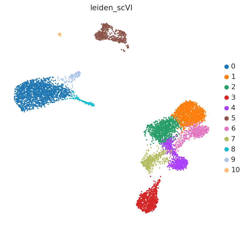
sc.pl.embedding(adata, "raw_counts_umap", color=["leiden_scVI"], frameon=False)

Color UMAP by topic proportions

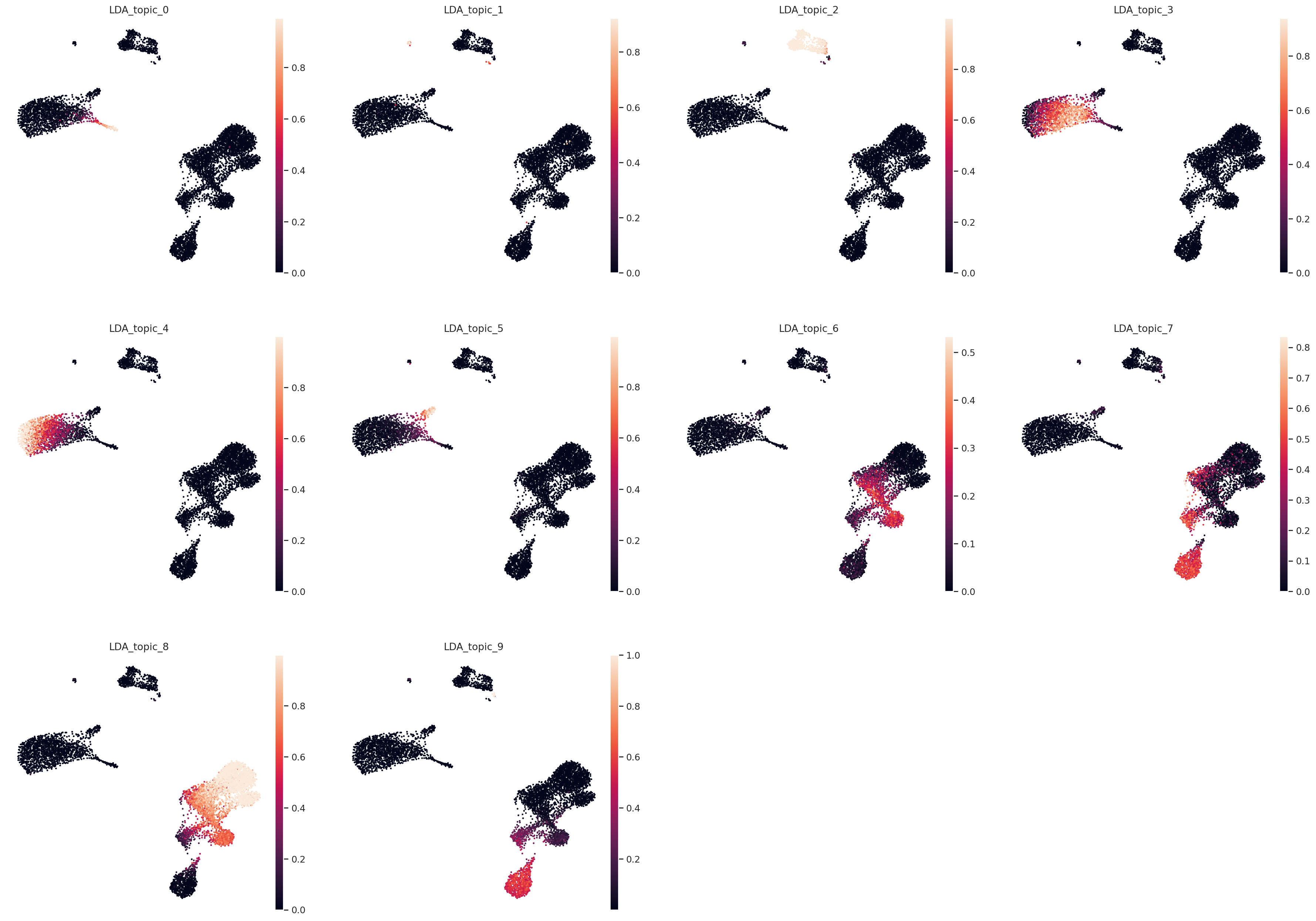
By coloring by UMAP by topic proportions, we find that the learned topics are generally dominant in cells close together in the UMAP space. In some cases, a topic is dominant in multiple clusters in the UMAP, which indicates similarilty between these clusters despite being far apart in the plot. This is not surprising considering that UMAP does not preserve local relationships beyond a certain threshold.

sc.pl.embedding(
    adata,
    "raw_counts_umap",
    color=[f"LDA_topic_{i}" for i in range(n_topics)],
    frameon=False,
)

Plot UMAP in topic space

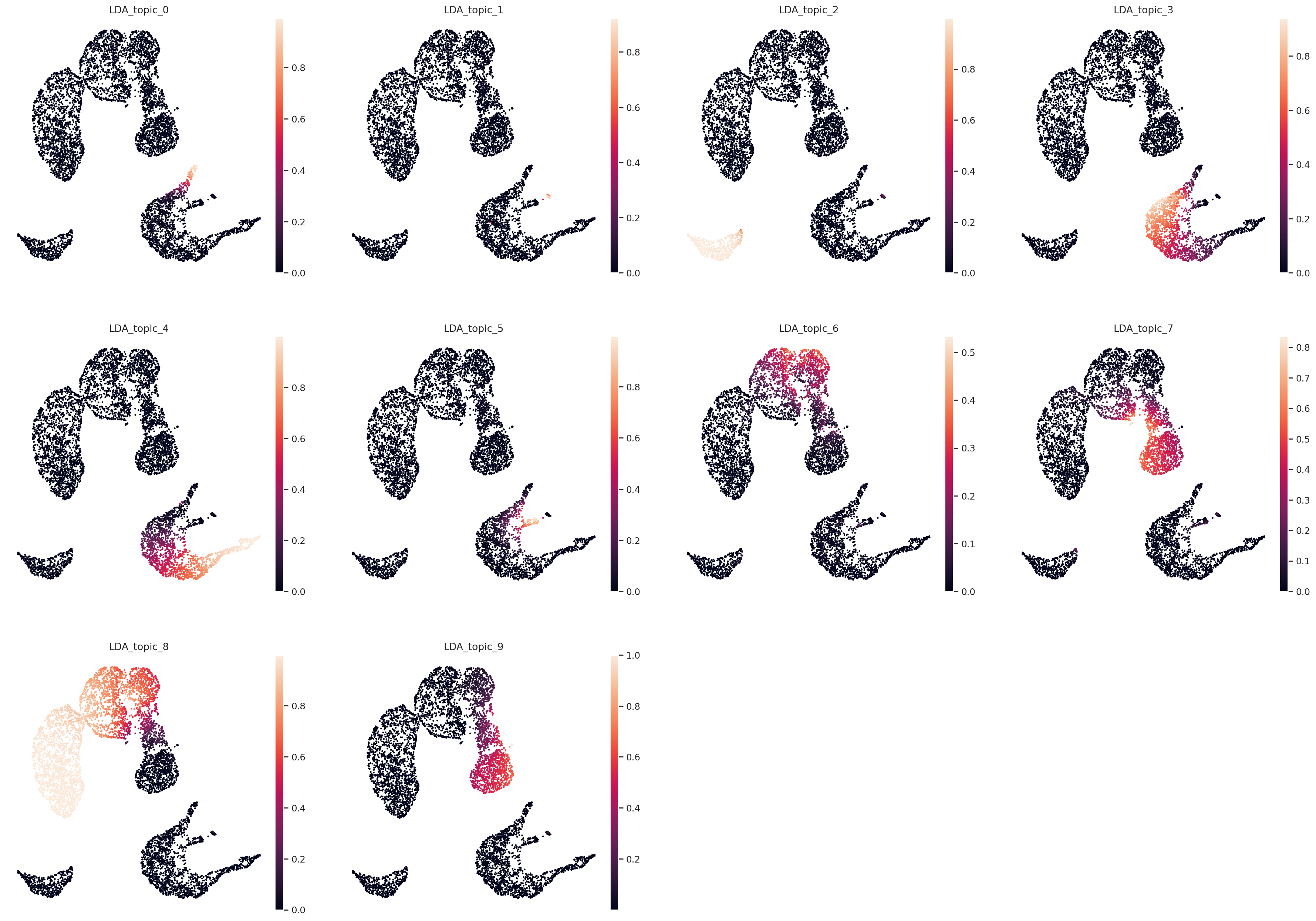
sc.pp.neighbors(adata, use_rep="X_LDA", n_neighbors=20, metric="hellinger")
sc.tl.umap(adata)

# Save UMAP to custom .obsm field.
adata.obsm["topic_space_umap"] = adata.obsm["X_umap"].copy()

sc.pl.embedding(
    adata,
    "topic_space_umap",
    color=[f"LDA_topic_{i}" for i in range(n_topics)],
    frameon=False,
)

Find top genes per topic

Similar to the topic proportions, model.get_feature_by_topic() returns a Monte Carlo estimate of the gene by topic matrix, which contains the proportion that a gene is weighted in each topic. This is also due to another approximation of the Dirichlet with a logistic-Normal distribution. We can inspect each topic in this matrix and sort by proportion allocated to each gene to determine top genes characterizing each topic.

feature_by_topic = model.get_feature_by_topic()
feature_by_topic.head()

	topic_0	topic_1	topic_2	topic_3	topic_4	topic_5	topic_6	topic_7	topic_8	topic_9
index
AL645608.8	0.000036	0.000023	0.000004	0.000001	2.783311e-06	0.000002	0.000006	0.000003	0.000001	0.000003
HES4	0.000733	0.000028	0.000013	0.000007	8.456480e-06	0.000010	0.000011	0.000005	0.000007	0.000005
ISG15	0.000720	0.000040	0.000413	0.000472	2.592755e-04	0.000133	0.001524	0.002357	0.001094	0.000327
TNFRSF18	0.000004	0.000148	0.000035	0.000001	8.430371e-07	0.000002	0.000354	0.000023	0.000359	0.000138
TNFRSF4	0.000004	0.000056	0.000007	0.000001	1.509900e-06	0.000004	0.000271	0.000035	0.000835	0.000026

rank_by_topic = pd.DataFrame()
for i in range(n_topics):
    topic_name = f"topic_{i}"
    topic = feature_by_topic[topic_name].sort_values(ascending=False)
    rank_by_topic[topic_name] = topic.index
    rank_by_topic[f"{topic_name}_prop"] = topic.values

rank_by_topic.head()

	topic_0	topic_0_prop	topic_1	topic_1_prop	topic_2	topic_2_prop	topic_3	topic_3_prop	topic_4	topic_4_prop	topic_5	topic_5_prop	topic_6	topic_6_prop	topic_7	topic_7_prop	topic_8	topic_8_prop	topic_9	topic_9_prop
0	FTL	0.114418	CD74	0.061230	CD74	0.108184	FTH1	0.059314	S100A9	0.143670	HLA-DRA	0.085101	S100A4	0.161333	ACTB	0.208307	TMSB4X	0.139633	GNLY	0.107086
1	ACTB	0.068806	ACTB	0.037643	IGKC	0.065732	FTL	0.057074	S100A8	0.099610	CD74	0.081020	SH3BGRL3	0.042521	TMSB4X	0.177480	TMSB10	0.095124	NKG7	0.078788
2	TMSB4X	0.059545	FTH1	0.028644	HLA-DRA	0.059559	LYZ	0.056565	LYZ	0.057241	ACTB	0.059655	S100A6	0.039614	TMSB10	0.079250	ACTB	0.094564	IGKC	0.077853
3	FTH1	0.059212	TMSB4X	0.025981	TMSB4X	0.043953	ACTB	0.035131	FTL	0.042915	HLA-DRB1	0.050423	ANXA1	0.037930	ACTG1	0.051750	JUNB	0.033868	CCL5	0.054798
4	S100A4	0.029395	CYBA	0.020130	TMSB10	0.041685	TMSB4X	0.035055	ACTB	0.038939	TMSB4X	0.042672	DUSP1	0.037028	S100A4	0.047518	FTL	0.029890	IGLC2	0.051152