Model hyperparameter tuning with scVI

Warning

scvi.autotune development is still in progress. The API is subject to change.

Finding an effective set of model hyperparameters (e.g. learning rate, number of hidden layers, etc.) is an important component in training a model as its performance can be highly dependent on these non-trainable parameters. Manually tuning a model often involves picking a set of hyperparameters to search over and then evaluating different configurations over a validation set for a desired metric. This process can be time consuming and can require some prior intuition about a model and dataset pair, which is not always feasible.

In this tutorial, we show how to use scvi’s autotune module, which allows us to automatically find a good set of model hyperparameters using Ray Tune. We will use SCVI and a subsample of the heart cell atlas for the task of batch correction, but the principles outlined here can be applied to any model and dataset. In particular, we will go through the following steps:

1. Installing required packages

2. Loading and preprocessing the dataset

3. Defining the tuner and discovering hyperparameters

4. Running the tuner

5. Comparing latent spaces

6. Optional: Monitoring progress with Tensorboard

7. Optional: Tuning over integration metrics with scib-metrics

Installing required packages

Note

Running the following cell will install tutorial dependencies on Google Colab only. It will have no effect on environments other than Google Colab.

!pip install --quiet scvi-colab
from scvi_colab import install

install()

WARNING: Running pip as the 'root' user can result in broken permissions and conflicting behaviour with the system package manager, possibly rendering your system unusable. It is recommended to use a virtual environment instead: https://pip.pypa.io/warnings/venv. Use the --root-user-action option if you know what you are doing and want to suppress this warning.

[notice] A new release of pip is available: 25.0.1 -> 26.1.2
[notice] To update, run: pip install --upgrade pip

import os
import tempfile

import ray
import scanpy as sc
import scvi
import seaborn as sns
import torch
from ray import tune
from scvi import autotune

os.environ["JAX_PLATFORMS"] = "cpu"
os.environ["TUNE_DISABLE_STRICT_METRIC_CHECKING"] = "1"

scvi.settings.seed = 0
print("Last run with scvi-tools version:", scvi.__version__)

Last run with scvi-tools version: 1.5.0

Note

You can modify save_dir below to change where the data files for this tutorial are saved.

sc.set_figure_params(figsize=(6, 6), frameon=False)
sns.set_theme()
torch.set_float32_matmul_precision("high")
save_dir = tempfile.TemporaryDirectory()
scvi.settings.logging_dir = save_dir.name

%config InlineBackend.print_figure_kwargs={"facecolor": "w"}
%config InlineBackend.figure_format="retina"

Loading and preprocessing the dataset

adata = scvi.data.heart_cell_atlas_subsampled(save_path=save_dir.name)
adata.layers["counts"] = adata.X.copy()  # preserve counts
sc.pp.filter_genes(adata, min_counts=3)
adata

INFO     Downloading file at /tmp/tmpbobw85tn/hca_subsampled_20k.h5ad

AnnData object with n_obs × n_vars = 18641 × 26469
    obs: 'NRP', 'age_group', 'cell_source', 'cell_type', 'donor', 'gender', 'n_counts', 'n_genes', 'percent_mito', 'percent_ribo', 'region', 'sample', 'scrublet_score', 'source', 'type', 'version', 'cell_states', 'Used'
    var: 'gene_ids-Harvard-Nuclei', 'feature_types-Harvard-Nuclei', 'gene_ids-Sanger-Nuclei', 'feature_types-Sanger-Nuclei', 'gene_ids-Sanger-Cells', 'feature_types-Sanger-Cells', 'gene_ids-Sanger-CD45', 'feature_types-Sanger-CD45', 'n_counts'
    uns: 'cell_type_colors'
    layers: 'counts'

The only preprocessing step we will perform in this case will be to subsample the dataset for 2000 highly variable genes using scanpy for faster model training.

adata.layers["counts"] = adata.X.copy()  # preserve counts
sc.pp.normalize_total(adata, target_sum=1e4)
sc.pp.log1p(adata)
adata.raw = adata  # freeze the state in `.raw`

sc.pp.highly_variable_genes(
    adata,
    n_top_genes=1200,
    subset=True,
    layer="counts",
    flavor="seurat_v3",
    batch_key="cell_source",
)
adata

AnnData object with n_obs × n_vars = 18641 × 1200
    obs: 'NRP', 'age_group', 'cell_source', 'cell_type', 'donor', 'gender', 'n_counts', 'n_genes', 'percent_mito', 'percent_ribo', 'region', 'sample', 'scrublet_score', 'source', 'type', 'version', 'cell_states', 'Used'
    var: 'gene_ids-Harvard-Nuclei', 'feature_types-Harvard-Nuclei', 'gene_ids-Sanger-Nuclei', 'feature_types-Sanger-Nuclei', 'gene_ids-Sanger-Cells', 'feature_types-Sanger-Cells', 'gene_ids-Sanger-CD45', 'feature_types-Sanger-CD45', 'n_counts', 'highly_variable', 'highly_variable_rank', 'means', 'variances', 'variances_norm', 'highly_variable_nbatches'
    uns: 'cell_type_colors', 'log1p', 'hvg'
    layers: 'counts'

Defining the tuner and discovering hyperparameters

The first part of our workflow is the same as the standard scvi-tools workflow: we start with our desired model class, and we register our dataset with it using setup_anndata. All datasets must be registered prior to hyperparameter tuning. It important that batch_key and labels_key will be explicitly defined to use it scib-autotune (later on).

model_cls = scvi.model.SCVI
model_cls.setup_anndata(
    adata,
    layer="counts",
    labels_key="cell_type",
    batch_key="cell_source",
    categorical_covariate_keys=["donor"],
    continuous_covariate_keys=["percent_mito", "percent_ribo"],
)

Our main entry point to the autotune module is the ModelTuner class, a wrapper around ray.tune.Tuner with additional functionality specific to scvi-tools. We can define a new ModelTuner by providing it with our model class.

ModelTuner will register all tunable hyperparameters in SCVI and all of them are accessible to tune starting version 1.2.0.

Running the tuner

Now that we know what hyperparameters are available to us, we can define a search space using the search space API in ray.tune. For this tutorial, we choose a simple search space with two model hyperparameters and one training plan hyperparameter. These can all be combined into a single dictionary that we pass into the fit method.

search_space = {
    "model_params": {"n_hidden": tune.choice([64, 128, 256]), "n_layers": tune.choice([1, 2, 3])},
    "train_params": {"max_epochs": 100, "plan_kwargs": {"lr": tune.loguniform(1e-4, 1e-2)}},
}

There are a couple more arguments we should be aware of before fitting the tuner:

• num_samples: The total number of hyperparameter sets to sample from ``. This is the total number of models that will be trained.

  For example, if we set num_samples=2, based on the above search space, we might sample two models with the following hyperparameter configurations:

  model1 = {
      "n_hidden": 64,
      "n_layers": 1,
      "lr": 0.001,
  }
  model2 = {
      "n_hidden": 64,
      "n_layers": 3,
      "lr": 0.0001,
  }
  

• max_epochs: The maximum number of epochs to train each model for.

  Note: This does not mean that each model will be trained for max_epochs. Depending on the scheduler used, some trials are likely to be stopped early.

• resources: A dictionary of maximum resources to allocate for the whole experiment. This allows us to run concurrent trials on limited hardware.

Now, we can call fit on the tuner to start the hyperparameter sweep. This will return a TuneAnalysis dataclass, which will contain the best set of hyperparameters, as well as other information.

ray.init(log_to_driver=False)

results = autotune.run_autotune(
    model_cls,
    data=adata,
    mode="min",
    metrics="validation_loss",
    search_space=search_space,
    num_samples=5,
    resources={"cpu": 10, "gpu": 1},
    ignore_reinit_error=True,
)

INFO     Running autotune experiment scvi_cb22c536-24b2-4297-aad1-30508672fa7d.

Tune Status

Current time:	2026-07-08 15:37:31
Running for:	00:04:59.57
Memory:	34.6/377.2 GiB

System Info

Using AsyncHyperBand: num_stopped=5
Bracket: Iter 64.000: -284.4673156738281 | Iter 32.000: -281.8278350830078 | Iter 16.000: -283.17088317871094 | Iter 8.000: -287.85008239746094 | Iter 4.000: -295.5080108642578 | Iter 2.000: -311.1089172363281 | Iter 1.000: -358.7673034667969
Logical resource usage: 10.0/64 CPUs, 1.0/1 GPUs (0.0/1.0 accelerator_type:RTX)

Trial Status

Trial name	status	loc	model_params/n_hidde n	model_params/n_layer s	train_params/max_epo chs	train_params/plan_kw args/lr	iter	total time (s)	validation_loss
_trainable_01a760ce	TERMINATED	172.18.0.2:4146	128	1	100	0.000582248	100	64.4397	285.874
_trainable_2049011c	TERMINATED	172.18.0.2:4338	256	3	100	0.00253497	64	47.9179	284.82
_trainable_6907f483	TERMINATED	172.18.0.2:4429	128	2	100	0.00146047	100	68.8898	285.11
_trainable_e089dd49	TERMINATED	172.18.0.2:4523	64	2	100	0.000402269	1	1.36079	499.254
_trainable_73f1d84c	TERMINATED	172.18.0.2:4609	256	3	100	0.00314606	64	47.926	284.609

Trial Progress

Trial name	checkpoint_dir_name	date	done	hostname	iterations_since_restore	node_ip	pid	time_since_restore	time_this_iter_s	time_total_s	timestamp	training_iteration	trial_id	validation_loss
_trainable_01a760ce		2026-07-08_15-33-50	True	78f939722389	100	172.18.0.2	4146	64.4397	0.624851	64.4397	1783524830	100	01a760ce	285.874
_trainable_2049011c		2026-07-08_15-34-51	True	78f939722389	64	172.18.0.2	4338	47.9179	0.737107	47.9179	1783524891	64	2049011c	284.82
_trainable_6907f483		2026-07-08_15-36-14	True	78f939722389	100	172.18.0.2	4429	68.8898	0.663724	68.8898	1783524974	100	6907f483	285.11
_trainable_73f1d84c		2026-07-08_15-37-31	True	78f939722389	64	172.18.0.2	4609	47.926	0.750636	47.926	1783525051	64	73f1d84c	284.609
_trainable_e089dd49		2026-07-08_15-36-29	True	78f939722389	1	172.18.0.2	4523	1.36079	1.36079	1.36079	1783524989	1	e089dd49	499.254

print(results.result_grid)

ResultGrid<[
  Result(
    metrics={'validation_loss': 285.8740234375},
    path='/tmp/tmpbobw85tn/scvi_cb22c536-24b2-4297-aad1-30508672fa7d/scvi_cb22c536-24b2-4297-aad1-30508672fa7d/_trainable_01a760ce_1_n_hidden=128,n_layers=1,max_epochs=100,lr=0.0006_2026-07-08_15-32-31',
    filesystem='local',
    checkpoint=None
  ),
  Result(
    metrics={'validation_loss': 284.8199462890625},
    path='/tmp/tmpbobw85tn/scvi_cb22c536-24b2-4297-aad1-30508672fa7d/scvi_cb22c536-24b2-4297-aad1-30508672fa7d/_trainable_2049011c_2_n_hidden=256,n_layers=3,max_epochs=100,lr=0.0025_2026-07-08_15-32-45',
    filesystem='local',
    checkpoint=None
  ),
  Result(
    metrics={'validation_loss': 285.1097412109375},
    path='/tmp/tmpbobw85tn/scvi_cb22c536-24b2-4297-aad1-30508672fa7d/scvi_cb22c536-24b2-4297-aad1-30508672fa7d/_trainable_6907f483_3_n_hidden=128,n_layers=2,max_epochs=100,lr=0.0015_2026-07-08_15-34-03',
    filesystem='local',
    checkpoint=None
  ),
  Result(
    metrics={'validation_loss': 499.2536315917969},
    path='/tmp/tmpbobw85tn/scvi_cb22c536-24b2-4297-aad1-30508672fa7d/scvi_cb22c536-24b2-4297-aad1-30508672fa7d/_trainable_e089dd49_4_n_hidden=64,n_layers=2,max_epochs=100,lr=0.0004_2026-07-08_15-35-05',
    filesystem='local',
    checkpoint=None
  ),
  Result(
    metrics={'validation_loss': 284.6092834472656},
    path='/tmp/tmpbobw85tn/scvi_cb22c536-24b2-4297-aad1-30508672fa7d/scvi_cb22c536-24b2-4297-aad1-30508672fa7d/_trainable_73f1d84c_5_n_hidden=256,n_layers=3,max_epochs=100,lr=0.0031_2026-07-08_15-36-28',
    filesystem='local',
    checkpoint=None
  )
]>

Monitoring progress with Tensorboard

Ray by default plots the metrics and results into tensorboard. It can be accessed usually under http://localhost:6006/ once the optimization is done

Tuning over integration metrics with scib-metrics

Starting SCVI-Tools v1.3 we are now able to hyperparameter tune for optimal scib-metrics of any choice. This is currently works only for SCVI and SCANVI models.

The idea in performing this is very much the same as before, we just need to select a metric that can be optimize from the pool of metrics that scib-metrics holds as seen in the following list: “Silhouette label”, “Silhouette batch/BRAS”, “Isolated labels”, “Leiden NMI”, “Leiden ARI”, “KMeans NMI”, “KMeans ARI”, “cLISI”, “iLISI”, “KBET”, “Graph connectivity”, “PCR comparison”, “Batch correction”, “Bio conservation”, “Total” The last 3 are the aggegative metrics that are average of the relevant group.

Those metrics are the columns names of the output result table of scib metrics. For all metrics, higher means better and range [0..1]. For more information about those metrics see the scib-metric docs

Note that usually in order to compare bio conservation metrics we need to apply a semi supervised model. Also note that in order to save run time we select a random number of cells to calculate the scib metrics. The default is 100 but it can be changed with the parameter scib_subsample_rows, like in the following example: Here we apply the hyper parameter tuning for the same model in the previous example, while optimizing for global batch correction metric, see here)

search_space_scib = {
    "model_params": {"n_hidden": tune.choice([64, 128, 256]), "n_layers": tune.choice([1, 2, 3])},
    "train_params": {"max_epochs": 100, "plan_kwargs": {"lr": tune.loguniform(1e-4, 1e-2)}},
}

results_scib = autotune.run_autotune(
    model_cls,
    data=adata,
    metrics="Batch correction",
    mode="max",
    search_space=search_space_scib,
    num_samples=2,
    seed=0,
    scheduler="asha",
    searcher="hyperopt",
    resources={"cpu": 20, "gpu": 0},
    scib_subsample_rows=10000,
    ignore_reinit_error=True,
    solver="randomized",
)

INFO     Running autotune experiment scvi_6e84e6d8-ad6b-41e6-b785-5522f184ed23.

Tune Status

Current time:	2026-07-08 15:41:07
Running for:	00:03:35.39
Memory:	34.7/377.2 GiB

System Info

Using AsyncHyperBand: num_stopped=0
Bracket: Iter 64.000: None | Iter 32.000: None | Iter 16.000: None | Iter 8.000: None | Iter 4.000: None | Iter 2.000: None | Iter 1.000: 0.582427442073822
Logical resource usage: 20.0/64 CPUs, 0/1 GPUs (0.0/1.0 accelerator_type:RTX)

Trial Status

Trial name	status	loc	model_params/n_hidde n	model_params/n_layer s	train_params/max_epo chs	train_params/plan_kw args/lr	iter	total time (s)	Batch correction
_trainable_d17935b7	TERMINATED	172.18.0.2:4737	128	1	100	0.000582248	1	182.282	0.532889
_trainable_419eeb53	TERMINATED	172.18.0.2:4866	256	3	100	0.00253497	1	189.059	0.631966

Trial Progress

Trial name	Batch correction	checkpoint_dir_name	date	done	experiment_tag	hostname	iterations_since_restore	node_ip	pid	time_since_restore	time_this_iter_s	time_total_s	timestamp	training_iteration	trial_id
_trainable_419eeb53	0.631966		2026-07-08_15-41-06	True	2_n_hidden=256,n_layers=3,max_epochs=100,lr=0.0025	78f939722389	1	172.18.0.2	4866	189.059	189.059	189.059	1783525266	1	419eeb53
_trainable_d17935b7	0.532889		2026-07-08_15-40-46	True	1_n_hidden=128,n_layers=1,max_epochs=100,lr=0.0006	78f939722389	1	172.18.0.2	4737	182.282	182.282	182.282	1783525246	1	d17935b7

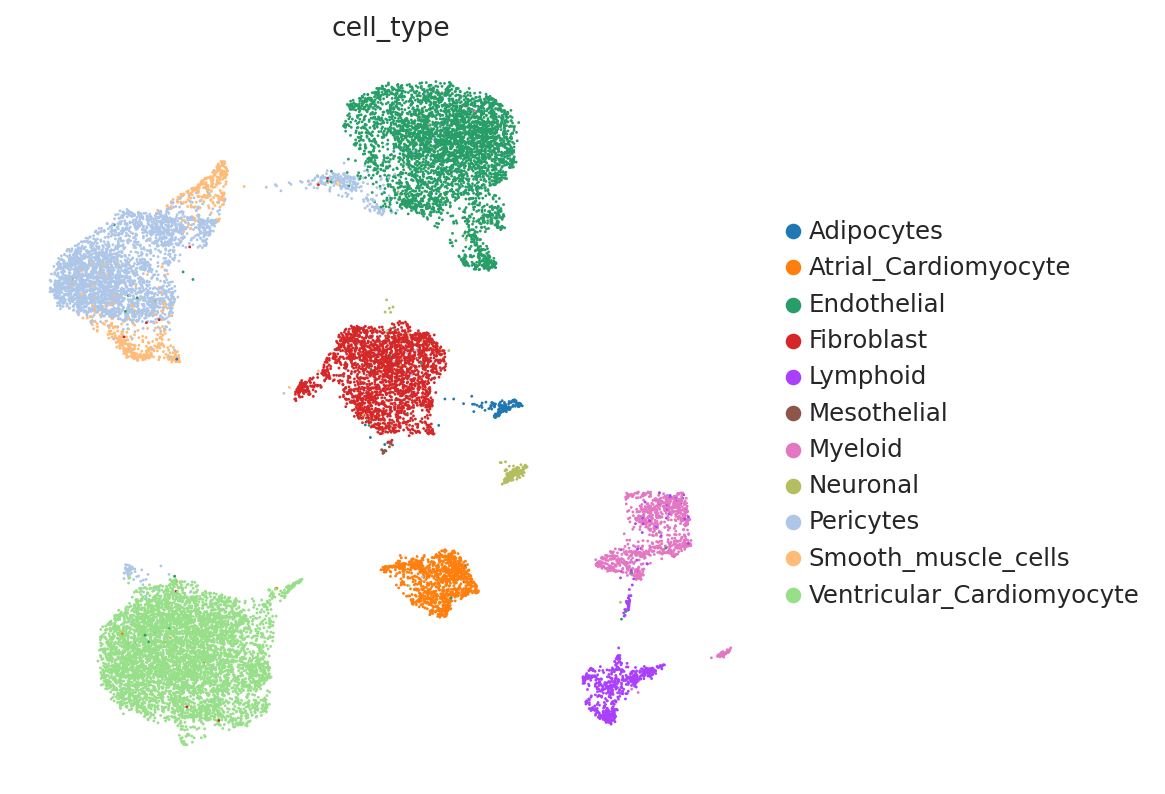
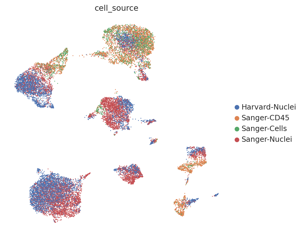
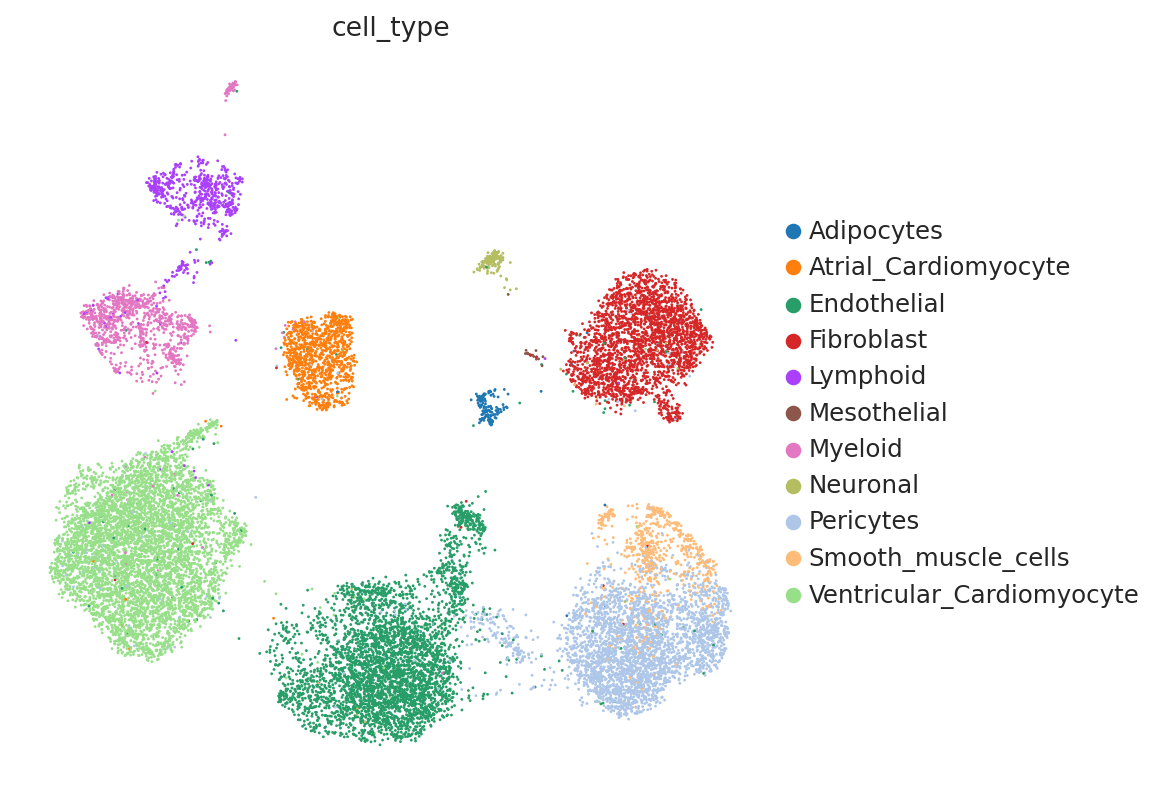
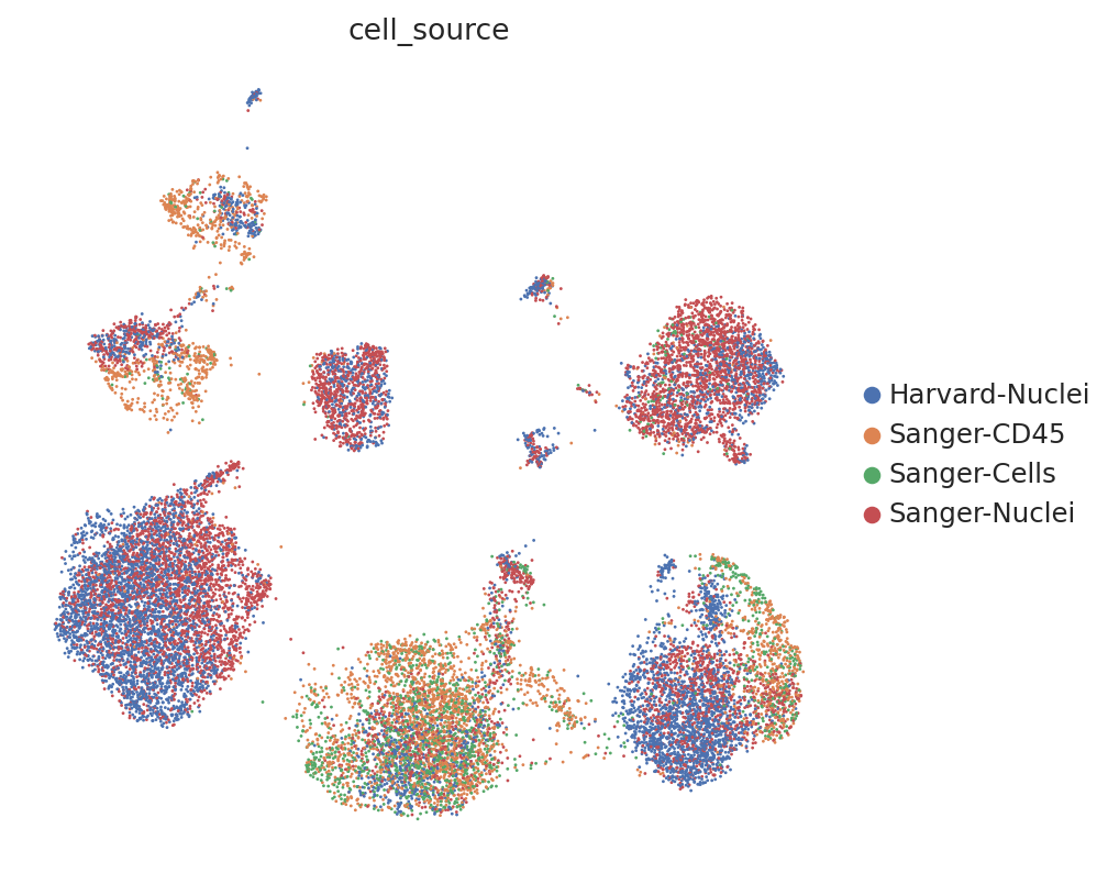
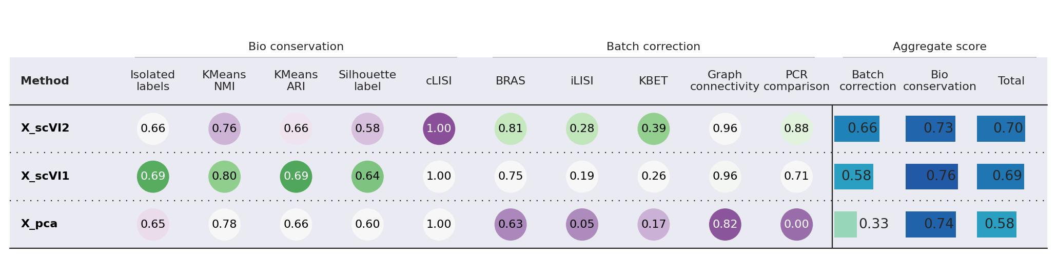
The second run ended with a higher score. We can visualize the different UMAPs to see that indeed the 2nd choice gives a better integration for cell source than the other:

model1 = scvi.model.SCVI(adata, n_hidden=128, n_layers=1)
model1.train(max_epochs=100, plan_kwargs={"lr": 0.0005})
adata.obsm["X_scVI1"] = model1.get_latent_representation()

sc.pp.neighbors(adata, use_rep="X_scVI1")
sc.tl.umap(adata, min_dist=0.3)
sc.pl.umap(
    adata,
    color=["cell_type"],
    frameon=False,
)
sc.pl.umap(
    adata,
    color=["cell_source"],
    ncols=2,
    frameon=False,
)

model2 = scvi.model.SCVI(adata, n_hidden=256, n_layers=3)
model2.train(max_epochs=100, plan_kwargs={"lr": 0.0025})
adata.obsm["X_scVI2"] = model2.get_latent_representation()

sc.pp.neighbors(adata, use_rep="X_scVI2")
sc.tl.umap(adata, min_dist=0.3)
sc.pl.umap(
    adata,
    color=["cell_type"],
    frameon=False,
)
sc.pl.umap(
    adata,
    color=["cell_source"],
    ncols=2,
    frameon=False,
)

# Manual Check:
from scib_metrics.benchmark import Benchmarker

bm = Benchmarker(
    adata,
    batch_key="cell_source",
    label_key="cell_type",
    embedding_obsm_keys=["X_pca", "X_scVI1", "X_scVI2"],
    n_jobs=-1,
)
bm.benchmark()

bm.plot_results_table(min_max_scale=False)

<plottable.table.Table at 0x74326f2d6060>