Disentangled representation learning with DRVI

DRVI (Moinfar & Theis, 2024) is an unsupervised deep generative model that learns an interpretable, disentangled latent representation of single-cell omics data. Disentanglement is induced in the decoder: the latent is split into distinct groups that are decoded separately and aggregated, so each factor tends to capture a distinct, biologically meaningful axis of variation.

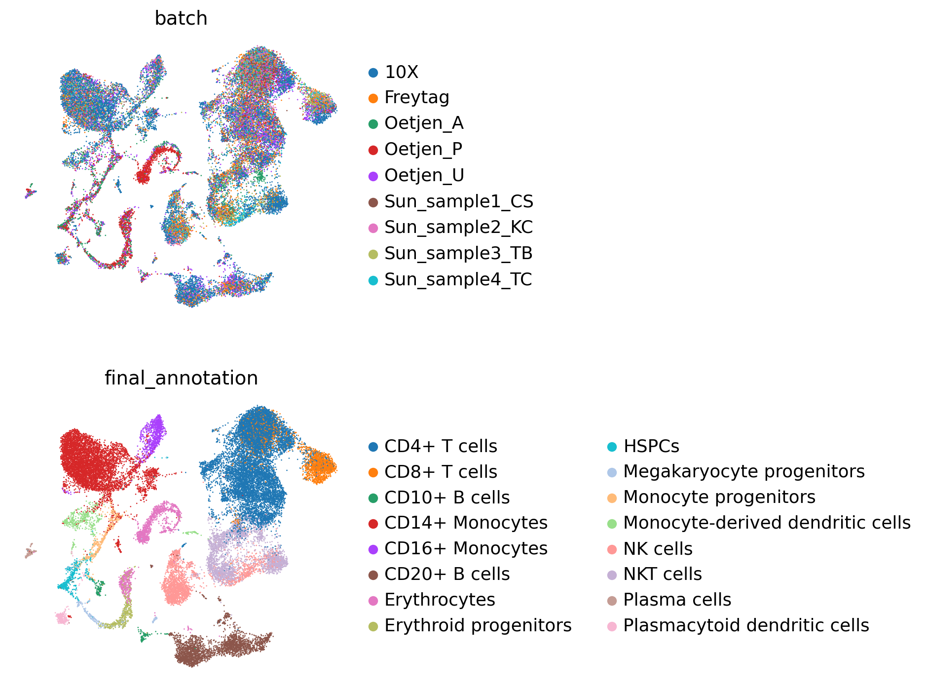
In this notebook we analyze an immune dataset of 9 batches from four human peripheral blood and bone marrow studies with 16 annotated cell types, training DRVI with 128 latent dimensions, to showcase:

• How to train DRVI

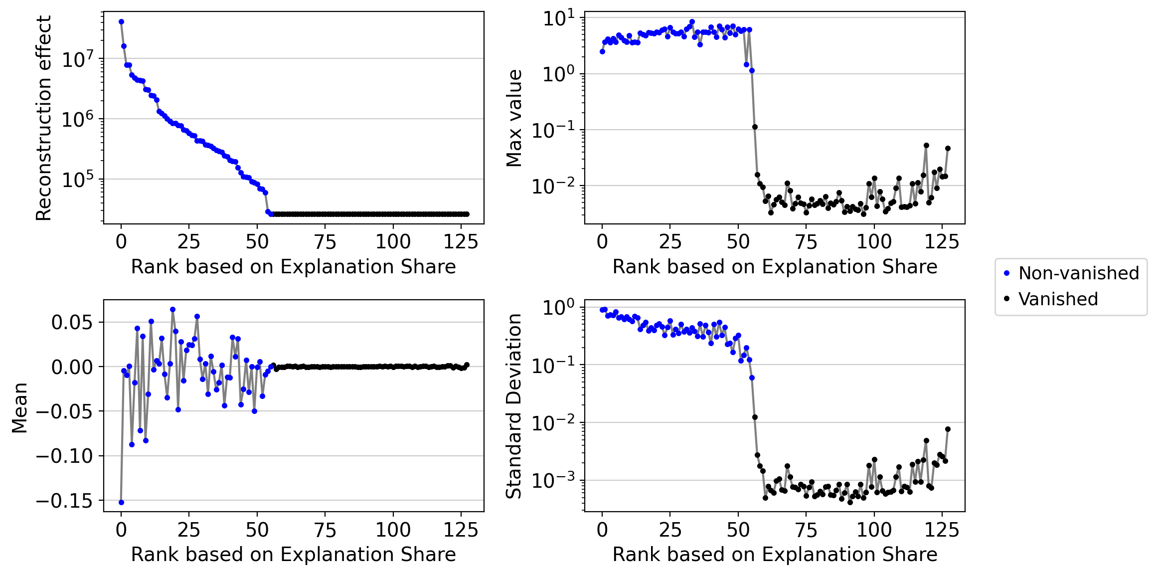
• How to inspect the latent space (vanished dimensions, UMAP, heatmap)

• How to run the interpretability pipeline and link latent dimensions to genes

The model in this tutorial is imported entirely from scvi-tools (scvi.external.DRVI). But the visualization helpers (drvi.utils.pl.*) come from the companion drvi-py package, installed with pip install drvi-py.

Note

Running the following cell is necessary if running in Google Colab.

!pip install --quiet scvi-colab
from scvi_colab import install

install()

[notice] A new release of pip is available: 24.3.1 -> 26.1.2
[notice] To update, run: pip install --upgrade pip

To install drvi-py package

!pip install --quiet drvi-py

Imports

import os
import tempfile
import warnings

warnings.filterwarnings("ignore")


import anndata as ad

# Helper functions from drvi-py package
import drvi
import scanpy as sc
import scvi
from matplotlib import pyplot as plt
from scvi.external import DRVI

scvi.settings.seed = 0
print("Last run with scvi-tools version:", scvi.__version__)
print("Last run with drvi version:", drvi.__version__)

Last run with scvi-tools version: 1.4.3
Last run with drvi version: 0.2.6

sc.set_figure_params(figsize=(4, 4), frameon=False)
save_dir = tempfile.TemporaryDirectory()
plt.rcParams["figure.dpi"] = 100
%config InlineBackend.print_figure_kwargs={'facecolor': 'w'}
%config InlineBackend.figure_format='retina'

Download and load data

We use the immune dataset (Luecken et al.) hosted on SCVERSE S3. The Villani batch is already removed because it contains non-count values, and 2000 batch-aware highly variable genes are selected.

adata_path = os.path.join(save_dir.name, "immune_hvg.h5ad")
adata = sc.read(
    adata_path, backup_url="https://exampledata.scverse.org/scvi-tools/Immune_HVG_human.h5ad"
)
adata

AnnData object with n_obs × n_vars = 32484 × 2000
    obs: 'batch', 'chemistry', 'data_type', 'dpt_pseudotime', 'final_annotation', 'mt_frac', 'n_counts', 'n_genes', 'sample_ID', 'size_factors', 'species', 'study', 'tissue'
    uns: 'batch_colors', 'final_annotation_colors', 'log1p', 'neighbors', 'pca', 'umap'
    obsm: 'X_pca', 'X_umap'
    varm: 'PCs'
    layers: 'counts'
    obsp: 'connectivities', 'distances'

Train DRVI

We register the count layer with scvi.external.DRVI.setup_anndata and train a model with 128 latent dimensions and two hidden layers of width 128 in both the encoder and the decoder. By default DRVI splits every latent dimension (n_split_latent = n_latent) with split_map splitting and logsumexp aggregation — the fully disentangled setting.

DRVI’s general hyperparameters are fully compatible with scVI (encoder width/depth, likelihood, covariate handling, and training arguments carry over directly). DRVI expects count data and uses a negative-binomial likelihood by default. Provide additional covariates via categorical_covariate_keys / continuous_covariate_keys in setup_anndata if needed. Depending on the data and modality, users can also choose other appropriate likelihoods such as Normal (needs library- and log-normalized data) or Poisson. Please refer to the API documentation for hyperparameter choices.

DRVI.setup_anndata(
    adata,
    layer="counts",
    batch_key="batch",
)

model = DRVI(
    adata,
    n_latent=128,
    n_hidden=128,
    n_layers=2,
    # depending on the variability of gene dispersions use 'gene' (default) or 'gene-batch'
    # dispersion='gene-batch',
)
model

INFO     The model has been initialized

Model with the following params:
  n_latent: 128
  n_split_latent: 128
  split_method: 'split_map'
  split_aggregation: 'logsumexp'. gene_likelihood: 'pnb'
Training status: Not Trained
Model's adata is minified?: False

n_epochs = 400
model.train(
    max_epochs=n_epochs,
    plan_kwargs={"n_epochs_kl_warmup": n_epochs},
)

Epoch 400/400: 100%|█████████████████████████████████████████████████████████████████████████████████████████████████████████████████████████████████████████████████████████████████| 400/400 [09:07<00:00,  1.37s/it, v_num=1, train_loss=745]
Epoch 400/400: 100%|█████████████████████████████████████████████████████████████████████████████████████████████████████████████████████████████████████████████████████████████████| 400/400 [09:07<00:00,  1.37s/it, v_num=1, train_loss=745]

model_path = os.path.join(save_dir.name, "drvi_model")
model.save(model_path, overwrite=True)
# model = DRVI.load(model_path, adata)

Latent space and interpretability scores

We store the latent representation in a new AnnData object (embed), where each factor is a latent dimension. DRVI.set_latent_dimension_stats annotates embed.var with per-dimension statistics (reconstruction effect, vanished status, ordering, min/max), and DRVI.calculate_interpretability_scores stores per-gene scores in embed.varm. The scores are calculated as follows:

• OOD (out-of-distribution): traverses each latent dimension through the decoder.

• IND (in-distribution): averages each dimension’s effect over the observed cells.

Note: The order of latent dimensions (DR 1, DR 2, …) is different from the order of columns in embed. Use embed.var['title'].

embed = ad.AnnData(model.get_latent_representation(), obs=adata.obs.copy())

model.set_latent_dimension_stats(embed, vanished_threshold=0.5)
model.calculate_interpretability_scores(embed, "OOD")
model.calculate_interpretability_scores(embed, "IND")

sc.pp.neighbors(embed, n_neighbors=10, use_rep="X", n_pcs=embed.X.shape[1])
sc.tl.umap(embed, spread=1.0, min_dist=0.5, random_state=123)
embed

AnnData object with n_obs × n_vars = 32484 × 128
    obs: 'batch', 'chemistry', 'data_type', 'dpt_pseudotime', 'final_annotation', 'mt_frac', 'n_counts', 'n_genes', 'sample_ID', 'size_factors', 'species', 'study', 'tissue', '_scvi_batch', '_scvi_labels'
    var: 'original_dim_id', 'reconstruction_effect', 'order', 'max_value', 'mean', 'min', 'max', 'std', 'std_abs', 'title', 'vanished', 'vanished_positive_direction', 'vanished_negative_direction'
    uns: 'neighbors', 'umap'
    obsm: 'X_umap'
    varm: 'OOD_min_possible_positive', 'OOD_min_possible_negative', 'OOD_max_possible_positive', 'OOD_max_possible_negative', 'OOD_combined_positive', 'OOD_combined_negative', 'IND_max_positive', 'IND_max_negative', 'IND_linear_weighted_mean_positive', 'IND_linear_weighted_mean_negative', 'IND_exp_weighted_mean_positive', 'IND_exp_weighted_mean_negative'
    obsp: 'distances', 'connectivities'

sc.pl.umap(embed, color=["batch", "final_annotation"], ncols=1, frameon=False)

Latent dimension stats

embed.var.sort_values("reconstruction_effect", ascending=False)[:5]

	original_dim_id	reconstruction_effect	order	max_value	mean	min	max	std	std_abs	title	vanished	vanished_positive_direction	vanished_negative_direction
120	120	41632488.0	0	2.483549	-0.152309	-2.483549	2.024353	0.904841	0.471779	DR 1	False	False	False
49	49	16319570.0	1	3.713669	-0.004452	-3.713669	1.571943	0.909893	0.590519	DR 2	False	False	False
17	17	7838704.5	2	4.173703	-0.009392	-4.173703	1.330191	0.713974	0.602237	DR 3	False	False	False
55	55	7814997.0	3	3.620830	0.000510	-3.620830	1.461988	0.733992	0.603089	DR 4	False	False	False
12	12	5391969.5	4	4.273345	-0.087206	-4.273345	1.702258	0.728451	0.522156	DR 5	False	False	False

drvi.utils.pl.plot_latent_dimension_stats(embed, ncols=2)

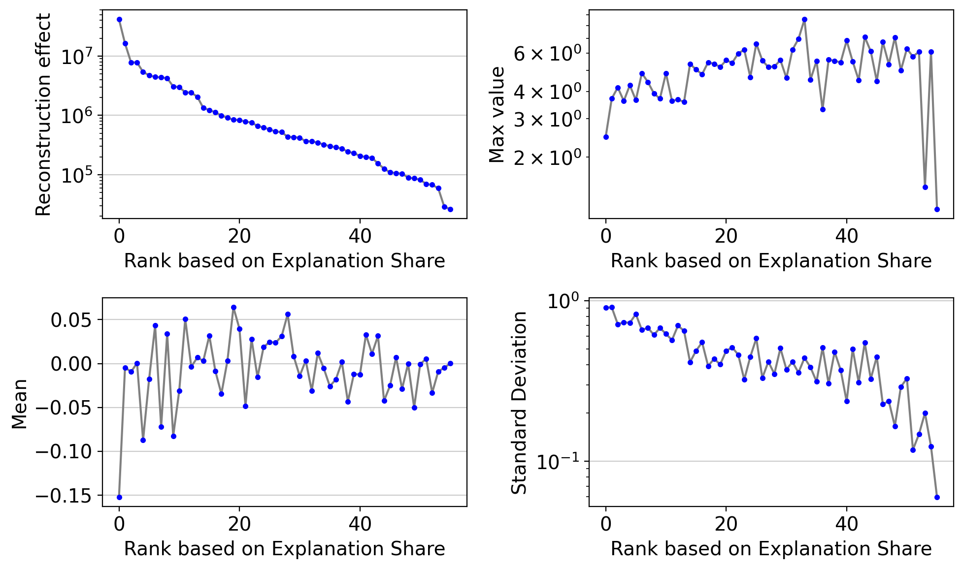
The same plot after removing vanished (inactive) dimensions:

drvi.utils.pl.plot_latent_dimension_stats(embed, ncols=2, remove_vanished=True)

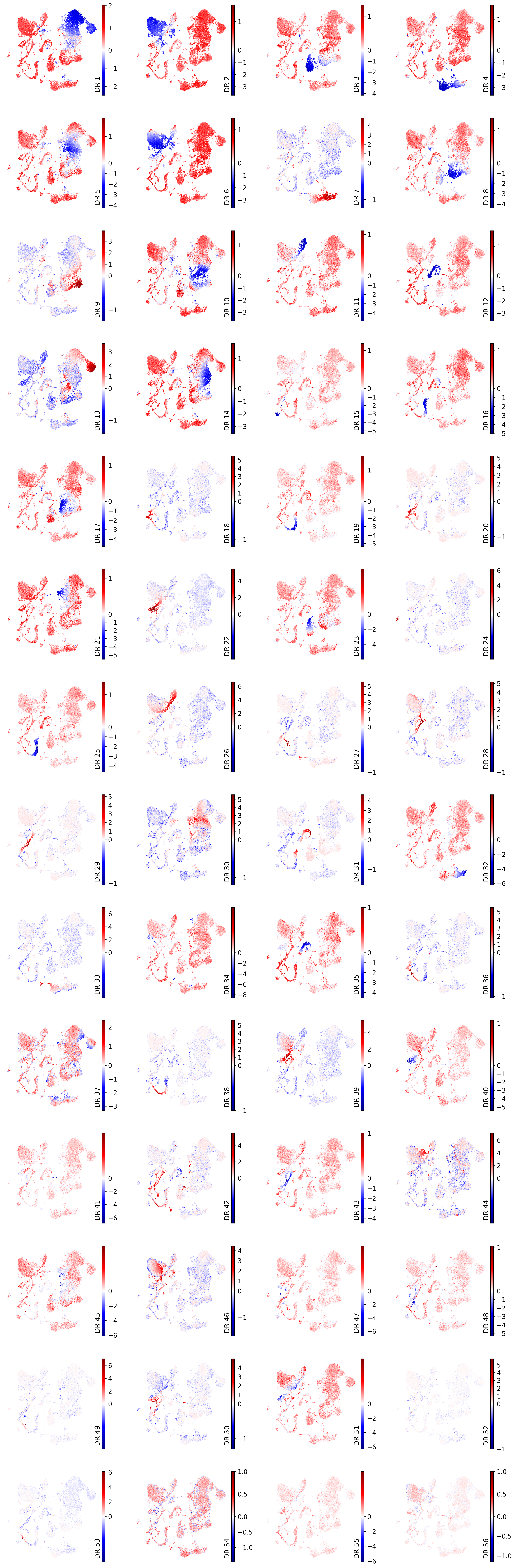
Plot latent dimensions

By default vanished dimensions are not plotted.

On the latent UMAP

drvi.utils.pl.plot_latent_dims_in_umap(embed)

As a heatmap

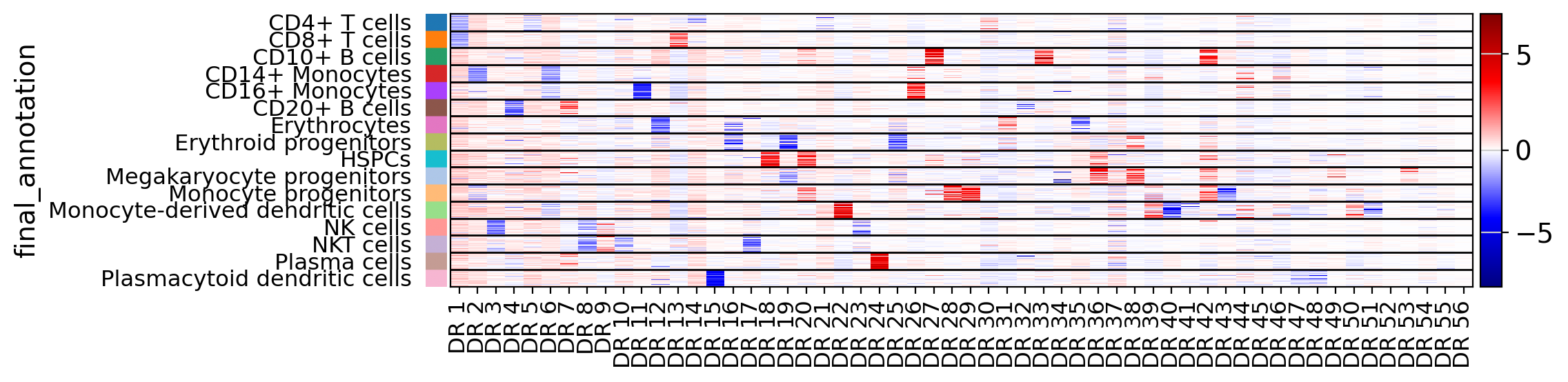
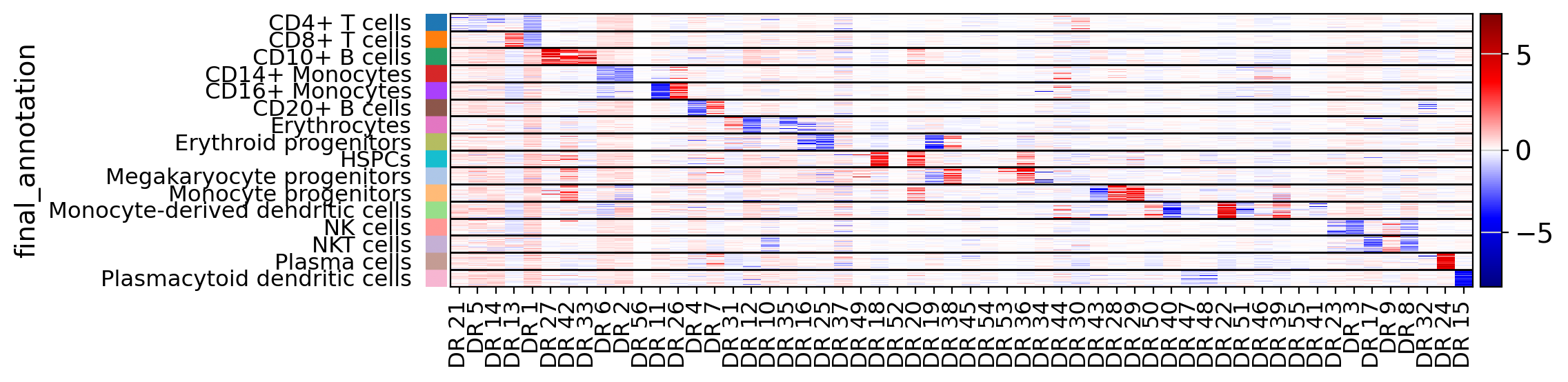
Heatmaps are useful to relate latent dimensions to known categories of the data. Dimensions can optionally be sorted by the category they are most relevant to.

drvi.utils.pl.plot_latent_dims_in_heatmap(embed, "final_annotation")

drvi.utils.pl.plot_latent_dims_in_heatmap(embed, "final_annotation", sort_by_categorical=True)

Interpretability

The per-gene scores were already computed above and live in embed.varm.

embed.varm

AxisArrays with keys: OOD_min_possible_positive, OOD_min_possible_negative, OOD_max_possible_positive, OOD_max_possible_negative, OOD_combined_positive, OOD_combined_negative, IND_max_positive, IND_max_negative, IND_linear_weighted_mean_positive, IND_linear_weighted_mean_negative, IND_exp_weighted_mean_positive, IND_exp_weighted_mean_negative

Out-of-distribution (OOD) scores

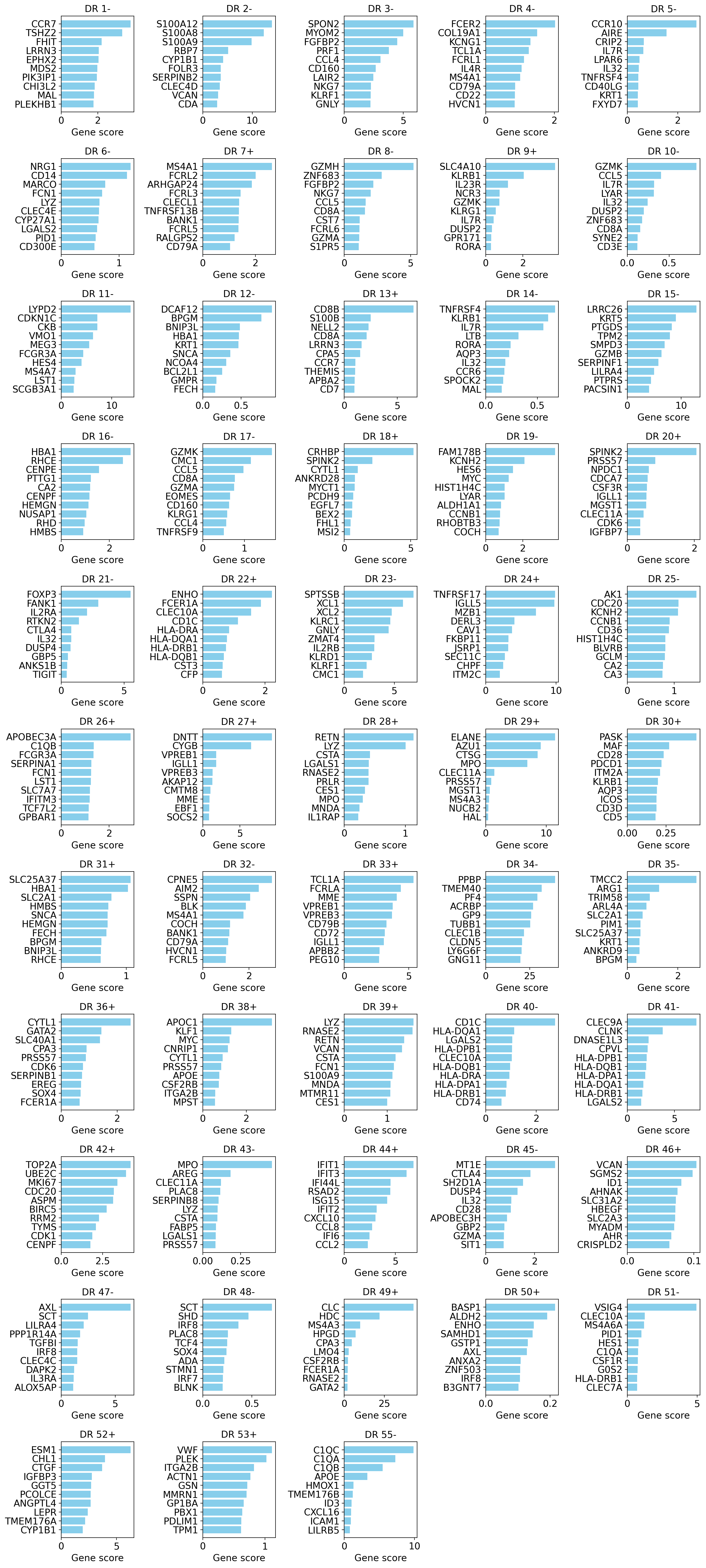
The default OOD_combined score combines the maximum effect and the specificity of each gene per dimension, which makes it our suggested score for finding the most specific genes of a program. If human-readable gene symbols live in a column of adata.var, pass it as gene_symbols=....

All scores can be obtained as a DataFrame (genes × dimensions). This includes all non-vanished dimensions / directions.

gene_scores_df = model.get_interpretability_scores(embed, adata)
gene_scores_df.iloc[:10, :10]

title	DR 1+	DR 1-	DR 2+	DR 2-	DR 3+	DR 3-	DR 4+	DR 4-	DR 5+	DR 5-
index
TCL1A	2.412687e-10	0.001456	5.522654e-11	0.000408	0.000000e+00	0.000791	5.305386e-12	1.257571	1.185880e-10	0.000328
IGLL5	8.337035e-13	0.000098	0.000000e+00	0.000146	0.000000e+00	0.000009	0.000000e+00	0.109184	0.000000e+00	0.000045
PTGDS	0.000000e+00	0.000579	3.385341e-12	0.000223	6.038034e-12	0.572757	6.456958e-09	0.000003	0.000000e+00	0.000644
GZMB	7.221287e-09	0.003130	4.590574e-09	0.000746	2.380274e-09	1.358150	4.744122e-08	0.000223	9.215202e-10	0.000249
PPBP	1.630017e-10	0.000183	1.078964e-09	0.000427	1.198929e-08	0.000013	6.093008e-09	0.000033	1.941316e-09	0.000007
CD79A	4.466629e-11	0.003331	3.197026e-08	0.000626	2.514043e-08	0.000338	1.575447e-10	0.856043	3.677643e-10	0.000492
FGFBP2	2.082743e-10	0.004022	7.083195e-10	0.000607	1.540659e-09	4.489642	7.033426e-10	0.001020	3.321929e-10	0.000340
FCGR3A	3.294372e-08	0.003072	1.656720e-09	0.002539	9.794753e-11	0.732972	5.033220e-09	0.000210	1.163810e-08	0.000223
GNLY	6.625820e-09	0.012571	1.878915e-09	0.002714	2.870239e-09	2.217784	2.881133e-08	0.002135	1.297420e-09	0.002112
GZMH	1.557257e-10	0.006391	8.314298e-10	0.000970	1.515572e-09	1.020924	8.565166e-10	0.000654	1.296662e-09	0.000201

drvi.utils.pl.plot_interpretability_scores(gene_scores_df, score_threshold=0.1)

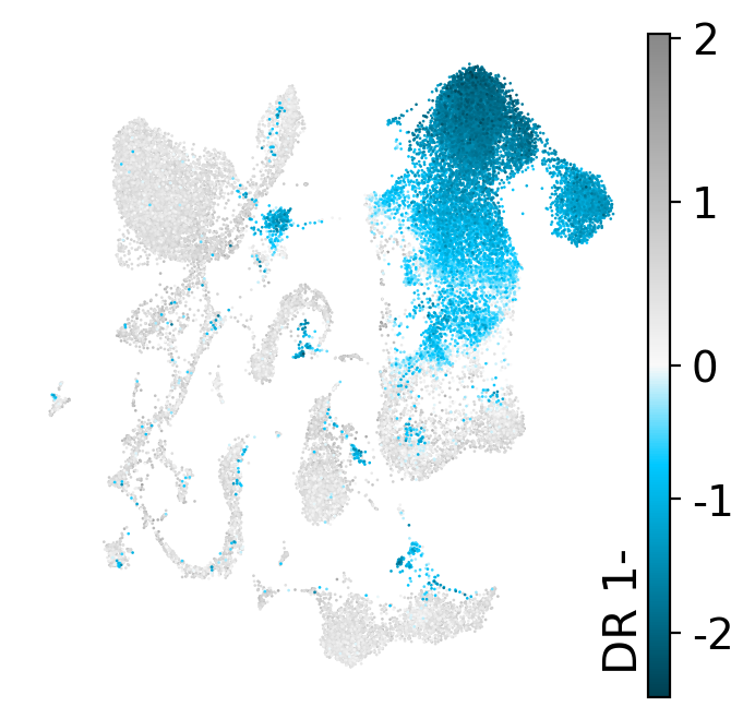
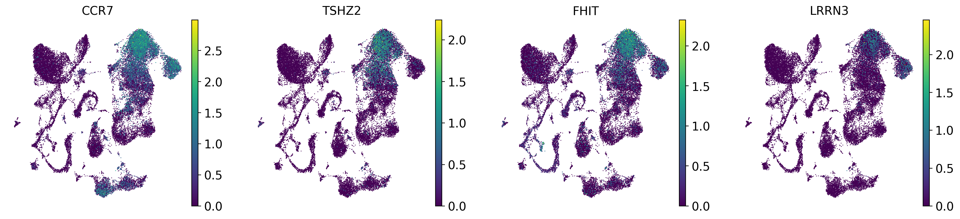
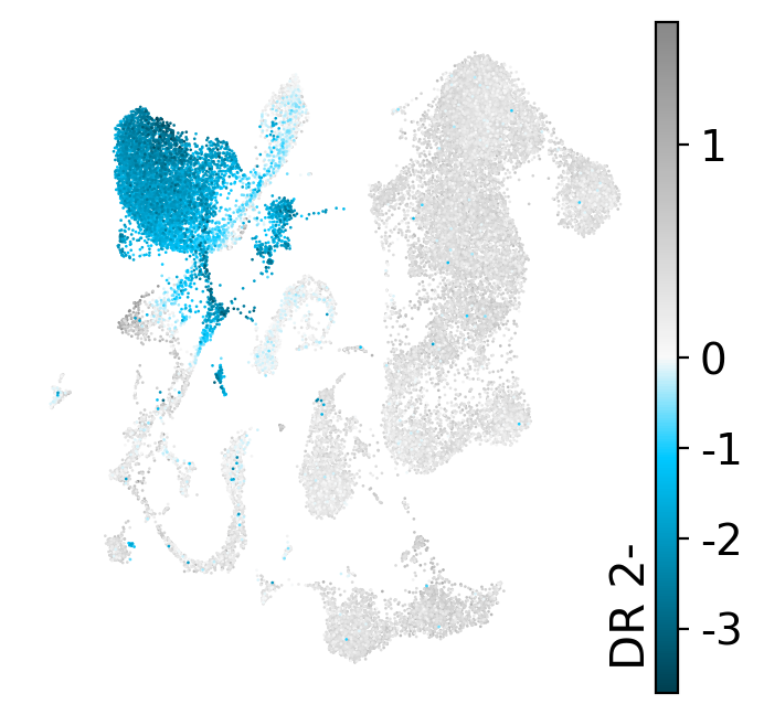
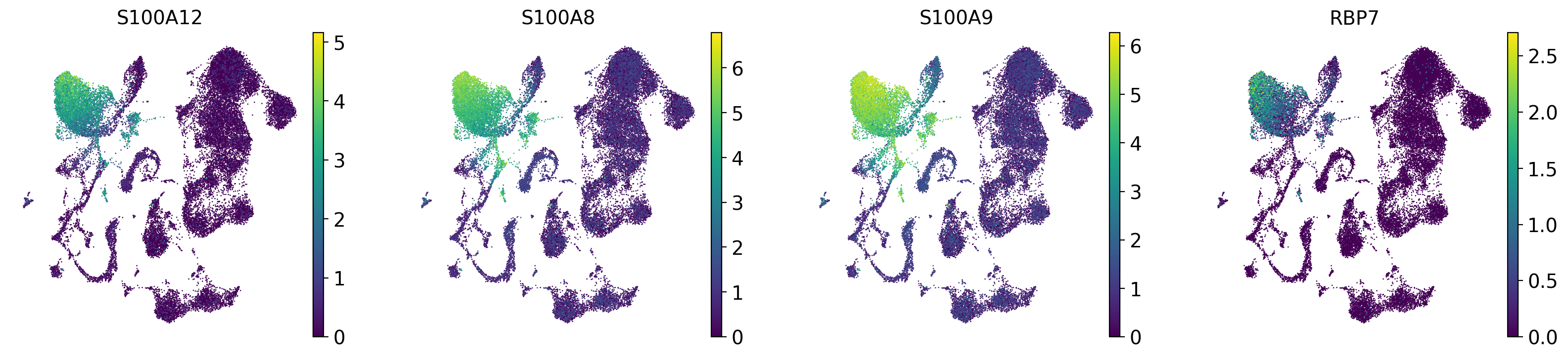
We can dig into individual dimensions: visualize a dimension on the UMAP (directional, so + and - are shown separately) and color the cells by its top genes. The exact dimension titles vary with the run and initialization.

# copy the latent UMAP onto the original (gene-level) AnnData
adata.obsm["X_drvi_umap"] = embed[adata.obs.index].obsm["X_umap"]

# We only show a few interpretable dimensions
for dim_title in gene_scores_df.columns[:4]:
    if gene_scores_df[dim_title].max() < 0.1:
        continue
    top_genes = gene_scores_df[dim_title].sort_values(ascending=False).index.to_list()[:4]
    print(dim_title)
    drvi.utils.pl.plot_latent_dims_in_umap(embed, dim_subset=[dim_title], directional=True)
    sc.pl.embedding(adata, "X_drvi_umap", color=top_genes, frameon=False)

DR 1-
DR 2-

In-distribution (IND) scores

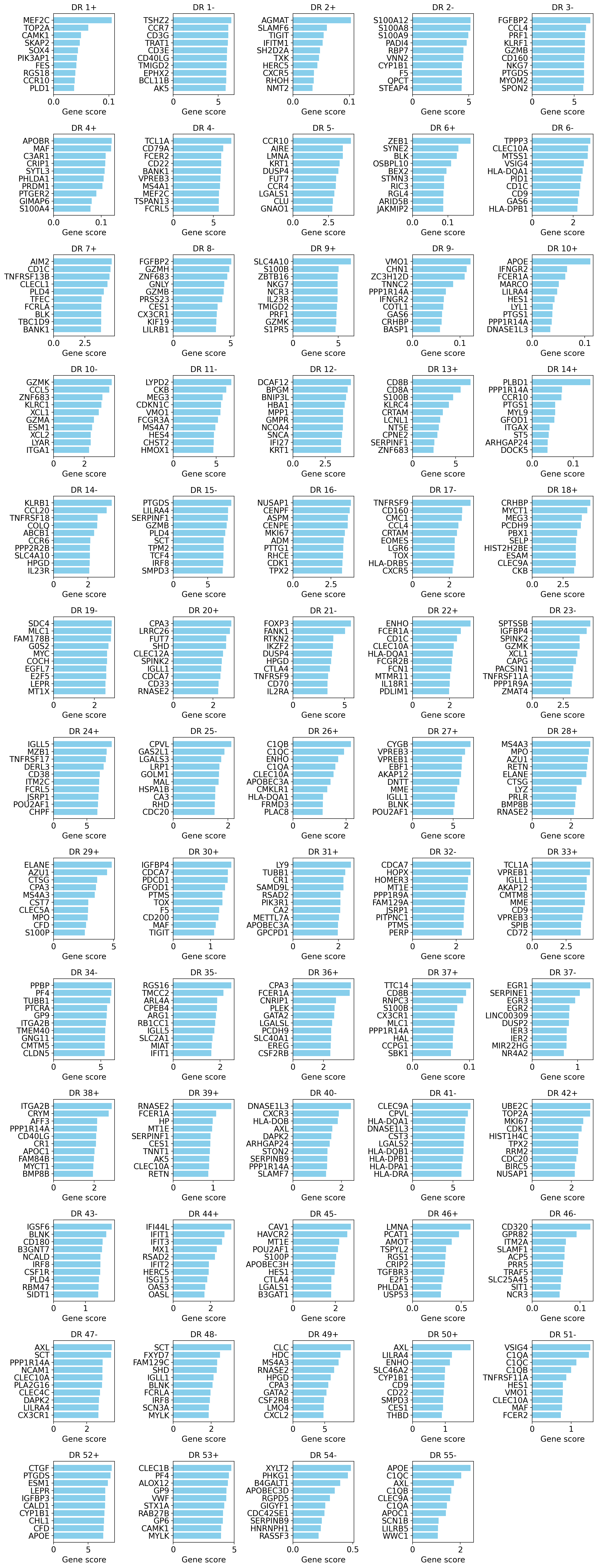
The IND scores average each dimension’s effect on each gene over all cells. Because genes are not filtered for uniqueness, broadly affected genes also keep high scores, giving a complete view of how each factor influences the transcriptome.

gene_scores_df_ind = model.get_interpretability_scores(
    embed, adata, key="IND_linear_weighted_mean"
)
gene_scores_df_ind.iloc[:10, :10]

title	DR 1+	DR 1-	DR 2+	DR 2-	DR 3+	DR 3-	DR 4+	DR 4-	DR 5+	DR 5-
index
TCL1A	0.005971	2.497063	0.001167	1.160384	0.001384	2.114294	0.000416	7.239596	0.002750	1.008309
IGLL5	0.000448	2.196086	0.000176	0.860792	0.000197	0.970224	0.000064	4.572513	0.000302	1.080758
PTGDS	0.000874	2.526320	0.000307	1.285834	0.000281	6.163900	0.005660	0.796921	0.000019	1.724263
GZMB	0.006450	2.521758	0.004755	1.187824	0.000510	6.265604	0.013632	1.810183	0.001139	0.799658
PPBP	0.004878	1.948129	0.000111	1.741534	0.012278	0.778982	0.010038	1.145155	0.004759	0.348709
CD79A	0.000977	3.127899	0.006475	1.488011	0.003377	1.750263	0.000041	6.236791	0.001201	0.870174
FGFBP2	0.000994	3.066175	0.000957	1.183964	0.000028	6.899695	0.000781	1.997372	0.000521	0.898678
FCGR3A	0.009571	2.601117	0.002131	1.532953	0.000113	6.004457	0.007521	1.132685	0.005178	0.658718
GNLY	0.002227	2.617745	0.000389	1.504693	0.000078	5.977234	0.005475	1.900974	0.000716	0.890538
GZMH	0.001197	2.238113	0.000904	1.064236	0.000088	5.464810	0.002496	1.482707	0.001472	0.594975

drvi.utils.pl.plot_interpretability_scores(gene_scores_df_ind)

Identification of programs

Once the top relevant genes of a dimension are known, the corresponding biological program can be identified using external information such as existing annotations, expert examination, gene-set enrichment analysis (GSEA), the literature, or automated annotation tools. Because this supervised information is never given to the model, the quality of the discovered signatures is neither affected nor biased by it — unidentified dimensions with high gene scores are promising candidates for further investigation.

More resources

This notebook covered the core DRVI workflow. For more:

• More tutorials — the DRVI documentation hosts additional tutorials (e.g. identification of rare cell types and mapping query data onto a DRVI reference): https://drvi.readthedocs.io/latest/tutorials/

• drvi-py package — beyond the plotting helpers used here, the companion drvi-py package (pip install drvi-py) provides more utility functions for latent-space analysis. See the API documentation for the full set of tools and plotting functions.