1. Introduction to single-cell Variational Inference (scVI)

In this introductory tutorial, we go through the different steps of a scVI workflow

1. Loading the data

2. Training the model

3. Retrieving the latent space and imputed values

4. Visualize the latent space with scanpy

5. Perform differential expression

6. Correcting batch effects with scVI

7. Miscenalleous information

# If running in Colab, navigate to Runtime -> Change runtime type
# and ensure you're using a Python 3 runtime with GPU hardware accelerator
# Installation of scVI in Colab can take several minutes

import sys
IN_COLAB = "google.colab" in sys.modules

def allow_notebook_for_test():
    print("Testing the basic tutorial notebook")

show_plot = True
test_mode = False
save_path = "data/"

if not test_mode:
    save_path = "../../data"

if IN_COLAB:
    !pip install --quiet scvi[notebooks]

import os
import numpy as np
import pandas as pd
import matplotlib.pyplot as plt
from scvi.dataset import CortexDataset, RetinaDataset
from scvi.models import VAE
from scvi.inference import UnsupervisedTrainer, load_posterior
from scvi import set_seed
import torch

# Control UMAP numba warnings
import warnings; warnings.simplefilter('ignore')

if IN_COLAB:
    %matplotlib inline

# Sets torch and numpy random seeds, run after all scvi imports
set_seed(0)

1.1. Loading data

Let us first load the CORTEX dataset described in Zeisel et al. (2015). scVI has many “built-in” datasets as well as support for loading arbitrary .csv, .loom, and .h5ad (AnnData) files. Please see our data loading Jupyter notebook for more examples of data loading.

• Zeisel, Amit, et al. “Cell types in the mouse cortex and hippocampus revealed by single-cell RNA-seq.” Science 347.6226 (2015): 1138-1142.

gene_dataset = CortexDataset(save_path=save_path, total_genes=None)
gene_dataset.subsample_genes(1000, mode="variance")
# we make the gene names lower case just for this tutorial
# scVI datasets preserve the case of the gene names as they are in the source files
gene_dataset.make_gene_names_lower()

[2020-01-29 07:41:10,549] INFO - scvi.dataset.dataset | File /data/expression.bin already downloaded
[2020-01-29 07:41:10,553] INFO - scvi.dataset.cortex | Loading Cortex data
[2020-01-29 07:41:19,357] INFO - scvi.dataset.cortex | Finished preprocessing Cortex data
[2020-01-29 07:41:19,790] INFO - scvi.dataset.dataset | Remapping labels to [0,N]
[2020-01-29 07:41:19,792] INFO - scvi.dataset.dataset | Remapping batch_indices to [0,N]
[2020-01-29 07:41:21,050] INFO - scvi.dataset.dataset | Downsampling from 19972 to 1000 genes
[2020-01-29 07:41:21,078] INFO - scvi.dataset.dataset | Computing the library size for the new data
[2020-01-29 07:41:21,090] INFO - scvi.dataset.dataset | Filtering non-expressing cells.
[2020-01-29 07:41:21,101] INFO - scvi.dataset.dataset | Computing the library size for the new data
[2020-01-29 07:41:21,106] INFO - scvi.dataset.dataset | Downsampled from 3005 to 3005 cells
[2020-01-29 07:41:21,107] INFO - scvi.dataset.dataset | Making gene names lower case

# Representation of the dataset object
gene_dataset

GeneExpressionDataset object with n_cells x nb_genes = 3005 x 1000
    gene_attribute_names: 'gene_names'
    cell_attribute_names: 'local_vars', 'local_means', 'batch_indices', 'precise_labels', 'labels'
    cell_categorical_attribute_names: 'labels', 'batch_indices'

In this demonstration and for this particular dataset, we use only 1000 genes as this dataset contains only 3005 cells. Furthermore, we select genes that have high variance across cells. By default, scVI uses an adapted version of the Seurat v3 vst gene selection and we recommend using this default mode.

Here are few practical rules for gene filtering with scVI:

• If many cells are available, it is in general better to use as many genes as possible. Of course, it might be of interest to remove ad-hoc genes depending on the downstream analysis or the application.

• When the dataset is small, it is usually better to filter out genes to avoid overfitting. In the original scVI publication, we reported poor imputation performance for when the number of cells was lower than the number of genes. This is all empirical and in general, it is hard to predict what the optimal number of genes will be.

• Generally, we advise relying on scanpy (and anndata) to load and preprocess data and then import the unnormalized filtered count matrix into scVI (see data loading tutorial). This can be done by putting the raw counts in adata.raw, or by using layers.

1.2. Training

• n_epochs: Number of epochs (passes through the entire dataset) to train the model. The number of epochs should be set according to the number of cells in your dataset. For example, 400 epochs is generally fine for < 10,000 cells. 200 epochs or fewer for greater than 10,000 cells. One should monitor the convergence of the training/test loss to determine the number of epochs necessary. For very large datasets (> 100,000 cells) you may only need ~10 epochs.

• lr: learning rate. Set to 0.001 here.

• use_cuda: Set to true to use CUDA (GPU required)

n_epochs = 400
lr = 1e-3
use_cuda = True

We now create the model and the trainer object. We train the model and output model likelihood every 5 epochs. In order to evaluate the likelihood on a test set, we split the datasets (the current code can also do train/validation/test, if a test_size is specified and train_size + test_size < 1, then the remaining cells get placed into a validation_set).

If a pre-trained model already exist in the save_path then load the same model rather than re-training it. This is particularly useful for large datasets.

train_size: In general, use a train_size of 1.0. We use 0.9 to monitor overfitting (ELBO on held-out data)

vae = VAE(gene_dataset.nb_genes)
trainer = UnsupervisedTrainer(
    vae,
    gene_dataset,
    train_size=0.90,
    use_cuda=use_cuda,
    frequency=5,
)

trainer.train(n_epochs=n_epochs, lr=lr)

training: 100%|██████████| 400/400 [01:53<00:00,  3.51it/s]

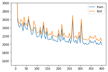
Plotting the likelihood change across the 500 epochs of training: blue for training error and orange for testing error.

elbo_train_set = trainer.history["elbo_train_set"]
elbo_test_set = trainer.history["elbo_test_set"]
x = np.linspace(0, 400, (len(elbo_train_set)))
plt.plot(x, elbo_train_set, label="train")
plt.plot(x, elbo_test_set, label="test")
plt.ylim(1500, 3000)
plt.legend()

<matplotlib.legend.Legend at 0x7fa4f35a3b00>

1.3. Obtaining the posterior object and sample latent space as well as imputation from it

The posterior object contains a model and a gene_dataset, as well as additional arguments that for Pytorch’s DataLoader. It also comes with many methods or utilities querying the model, such as differential expression, imputation and differential analyisis.

To get an ordered output result, we use the .sequential() posterior method, which returns another instance of posterior (with shallow copy of all its object references), but where the iteration is in the same ordered as its indices attribute.

full = trainer.create_posterior(trainer.model, gene_dataset, indices=np.arange(len(gene_dataset)))
# Updating the "minibatch" size after training is useful in low memory configurations
full = full.update({"batch_size":32})
latent, batch_indices, labels = full.sequential().get_latent()
batch_indices = batch_indices.ravel()

Similarly, it is possible to query the imputed values via the imputation method of the posterior object.

Imputation is an ambiguous term and there are two ways to perform imputation in scVI. The first way is to query the mean of the negative binomial distribution modeling the counts. This is referred to as sample_rate in the codebase and can be reached via the imputation method. The second is to query the normalized mean of the same negative binomial (please refer to the scVI manuscript). This is referred to as sample_scale in the codebase and can be reached via the get_sample_scale method. In differential expression for example, we of course rely on the normalized latent variable which is corrected for variations in sequencing depth.

imputed_values = full.sequential().imputation()
normalized_values = full.sequential().get_sample_scale()

The posterior object provides an easy way to save an experiment that includes not only the trained model, but also the associated data with the save_posterior and load_posterior tools.

1.3.1. Saving and loading results

# saving step (after training!)
save_dir = os.path.join(save_path, "full_posterior")
if not os.path.exists(save_dir):
    full.save_posterior(save_dir)

# loading step (in a new session)
retrieved_model = VAE(gene_dataset.nb_genes)  # uninitialized model
save_dir = os.path.join(save_path, "full_posterior")

retrieved_full = load_posterior(
    dir_path=save_dir,
    model=retrieved_model,
    use_cuda=use_cuda,
)

1.4. Visualizing the latent space with scanpy

scanpy is a handy and powerful python library for visualization and downstream analysis of single-cell RNA sequencing data. We show here how to feed the latent space of scVI into a scanpy object and visualize it using UMAP as implemented in scanpy. More on how scVI can be used with scanpy on this notebook. Note to advanced users: The code get_latent() returns only the mean of the posterior distribution for the latent space. However, we recover a full distribution with our inference framework. Let us keep in mind that the latent space visualized here is a practical summary of the data only. Uncertainty is needed for other downstream analyses such as differential expression.

import scanpy as sc
import anndata

post_adata = anndata.AnnData(X=gene_dataset.X)
post_adata.obsm["X_scVI"] = latent
post_adata.obs['cell_type'] = np.array([gene_dataset.cell_types[gene_dataset.labels[i][0]]
                                        for i in range(post_adata.n_obs)])
sc.pp.neighbors(post_adata, use_rep="X_scVI", n_neighbors=15)
sc.tl.umap(post_adata, min_dist=0.3)

fig, ax = plt.subplots(figsize=(7, 6))
sc.pl.umap(post_adata, color=["cell_type"], ax=ax, show=show_plot)

... storing 'cell_type' as categorical

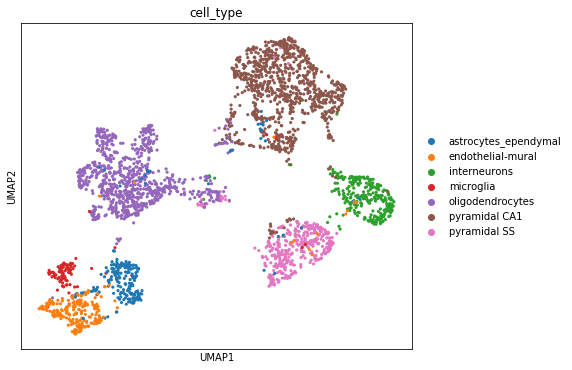
The user will note that we imported curated labels from the original publication. Our interface with scanpy makes it easy to cluster the data with scanpy from scVI’s latent space and then reinject them into scVI (e.g., for differential expression). We discuss this in the scanpy tutorial.

1.5. Differential Expression

From the trained VAE model we can sample the gene expression rate for each gene in each cell. For the two populations of interest, we can then randomly sample pairs of cells, one from each population to compare their expression rate for a gene. The degree of differential expression is measured by \(\text{logit}\frac{p}{(1-p)}\) where p is the probability of a cell from population A having a higher expression than a cell from population B. We can form the null distribution of the DE values by sampling pairs randomly from the combined population.

The following example is implemented for the cortext dataset, vary cell_types and genes_of_interest for other datasets.

1. Set population A and population B for comparison

cell_types = gene_dataset.cell_types
print(gene_dataset.cell_types)
# oligodendrocytes (#4) VS pyramidal CA1 (#5)
couple_celltypes = (4, 5)  # the couple types on which to study DE

print("\nDifferential Expression A/B for cell types\nA: %s\nB: %s\n" %
      tuple((cell_types[couple_celltypes[i]] for i in [0, 1])))

cell_idx1 = gene_dataset.labels.ravel() == couple_celltypes[0]
cell_idx2 = gene_dataset.labels.ravel() == couple_celltypes[1]

['astrocytes_ependymal' 'endothelial-mural' 'interneurons' 'microglia'
 'oligodendrocytes' 'pyramidal CA1' 'pyramidal SS']

Differential Expression A/B for cell types
A: oligodendrocytes
B: pyramidal CA1

2. Define parameters * n_samples: the number of times to sample px_scales from the vae model for each gene in each cell. * M_permutation: Number of pairs sampled from the px_scales values for comparison.

n_samples = 100
M_permutation = 100000

de_res = full.differential_expression_score(
    cell_idx1,
    cell_idx2,
    n_samples=n_samples,
    M_permutation=M_permutation,
)

3. Print out the differential expression value * bayes_factor: The bayes factor for cell type 1 having a higher expression than cell type 2 * proba_m1: The numerator of the bayes_factor quotient, the probability cell type 1 has higher expression than cell type 2 * proba_m2: The denominator of the bayes_factor quotient, equal to 1 minus proba_m1 * raw_meani: average UMI counts in cell type i * non_zeros_proportioni: proportion of non-zero expression in cell type i * raw_normalized_meani: average UMI counts in cell type i normalized by cell size * scalei: average scVI imputed gene expression scale in cell type i

genes_of_interest = ["thy1", "mbp"]
de_res.filter(items=genes_of_interest, axis=0)

	proba_m1	proba_m2	bayes_factor	scale1	scale2	raw_mean1	raw_mean2	non_zeros_proportion1	non_zeros_proportion2	raw_normalized_mean1	raw_normalized_mean2
thy1	0.01084	0.98916	-4.513612	0.000165	0.001225	0.589024	13.569755	0.219512	0.996805	0.089729	1.444312
mbp	0.99060	0.00940	4.657600	0.010763	0.000373	55.318295	2.787008	0.998780	0.452609	8.840034	0.298456

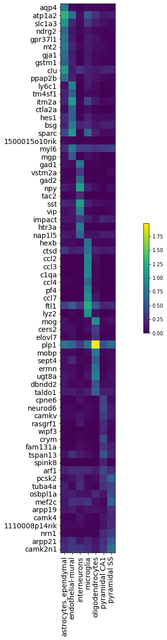
9. Visualize top 10 most expressed genes per cell types

per_cluster_de, cluster_id = full.one_vs_all_degenes(cell_labels=gene_dataset.labels.ravel(), min_cells=1)

markers = []
for x in per_cluster_de:
    markers.append(x[:10])
markers = pd.concat(markers)

genes = np.asarray(markers.index)
expression = [x.filter(items=genes, axis=0)['raw_normalized_mean1'] for x in per_cluster_de]
expression = pd.concat(expression, axis=1)
expression = np.log10(1 + expression)
expression.columns = gene_dataset.cell_types

plt.figure(figsize=(20, 20))
im = plt.imshow(expression, cmap='viridis', interpolation='none', aspect='equal')
ax = plt.gca()
ax.set_xticks(np.arange(0, 7, 1))
ax.set_xticklabels(gene_dataset.cell_types, rotation='vertical')
ax.set_yticklabels(genes)
ax.set_yticks(np.arange(0, 70, 1))
ax.tick_params(labelsize=14)
plt.colorbar(shrink=0.2)

<matplotlib.colorbar.Colorbar at 0x7fa49b3e3f28>

1.6. Correction for batch effects

We now load the RETINA dataset that is described in Shekhar et al. (2016) for an example of batch-effect correction. For more extensive utilization, we encourage the users to visit the harmonization as well as the annotation notebook which explain in depth how to deal with several datasets (in an unsupervised or semi-supervised fashion).

• Shekhar, Karthik, et al. “Comprehensive classification of retinal bipolar neurons by single-cell transcriptomics.” Cell 166.5 (2016): 1308-1323.

retina_dataset = RetinaDataset(save_path=save_path)

[2020-01-29 07:43:41,162] INFO - scvi.dataset.dataset | File /data/retina.loom already downloaded
[2020-01-29 07:43:41,163] INFO - scvi.dataset.loom | Preprocessing dataset
[2020-01-29 07:43:49,676] INFO - scvi.dataset.loom | Finished preprocessing dataset
[2020-01-29 07:43:51,455] INFO - scvi.dataset.dataset | Remapping labels to [0,N]
[2020-01-29 07:43:51,461] INFO - scvi.dataset.dataset | Remapping batch_indices to [0,N]

retina_dataset

GeneExpressionDataset object with n_cells x nb_genes = 19829 x 13166
    gene_attribute_names: 'gene_names'
    cell_attribute_names: 'labels', 'batch_indices', 'local_vars', 'local_means'
    cell_categorical_attribute_names: 'labels', 'batch_indices'

# Notice that the dataset has two batches
retina_dataset.batch_indices.ravel()[:10]

array([0, 0, 0, 0, 1, 0, 1, 1, 0, 0], dtype=uint16)

# Filter so that there are genes with at least 1 umi count in each batch separately
retina_dataset.filter_genes_by_count(per_batch=True)
# Run highly variable gene selection
retina_dataset.subsample_genes(4000)

[2020-01-29 07:43:51,834] INFO - scvi.dataset.dataset | Downsampling from 13166 to 13085 genes
[2020-01-29 07:43:52,732] INFO - scvi.dataset.dataset | Computing the library size for the new data
[2020-01-29 07:43:53,618] INFO - scvi.dataset.dataset | Filtering non-expressing cells.
[2020-01-29 07:43:54,345] INFO - scvi.dataset.dataset | Computing the library size for the new data
[2020-01-29 07:43:54,677] INFO - scvi.dataset.dataset | Downsampled from 19829 to 19829 cells
[2020-01-29 07:43:54,681] INFO - scvi.dataset.dataset | extracting highly variable genes

Transforming to str index.

[2020-01-29 07:44:10,054] INFO - scvi.dataset.dataset | Downsampling from 13085 to 4000 genes
[2020-01-29 07:44:11,878] INFO - scvi.dataset.dataset | Computing the library size for the new data
[2020-01-29 07:44:13,050] INFO - scvi.dataset.dataset | Filtering non-expressing cells.
[2020-01-29 07:44:14,119] INFO - scvi.dataset.dataset | Computing the library size for the new data
[2020-01-29 07:44:14,255] INFO - scvi.dataset.dataset | Downsampled from 19829 to 19829 cells

n_epochs = 200
lr = 1e-3
use_batches = True
use_cuda = True

# Train the model and output model likelihood every 10 epochs
# if n_batch = 0 then batch correction is not performed
# this is controlled by the use_batches boolean variable
vae = VAE(retina_dataset.nb_genes, n_batch=retina_dataset.n_batches * use_batches)
trainer = UnsupervisedTrainer(
    vae,
    retina_dataset,
    train_size=0.9 if not test_mode else 0.5,
    use_cuda=use_cuda,
    frequency=10,
)
trainer.train(n_epochs=n_epochs, lr=lr)

[2020-01-29 07:44:15,101] INFO - scvi.inference.inference | KL warmup phase exceeds overall training phaseIf your applications rely on the posterior quality, consider training for more epochs or reducing the kl warmup.
training: 100%|██████████| 200/200 [06:21<00:00,  1.91s/it]
[2020-01-29 07:50:36,512] INFO - scvi.inference.inference | Training is still in warming up phase. If your applications rely on the posterior quality, consider training for more epochs or reducing the kl warmup.

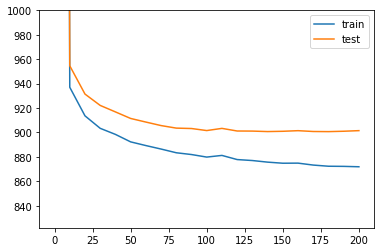
# Plotting the likelihood change across the 400 epochs of training:
# blue for training error and orange for testing error.

elbo_train = trainer.history["elbo_train_set"]
elbo_test = trainer.history["elbo_test_set"]
x = np.linspace(0, 200, (len(elbo_train)))
plt.plot(x, elbo_train, label="train")
plt.plot(x, elbo_test, label="test")
plt.ylim(min(elbo_train)-50, 1000)
plt.legend()

<matplotlib.legend.Legend at 0x7fa49ba344a8>

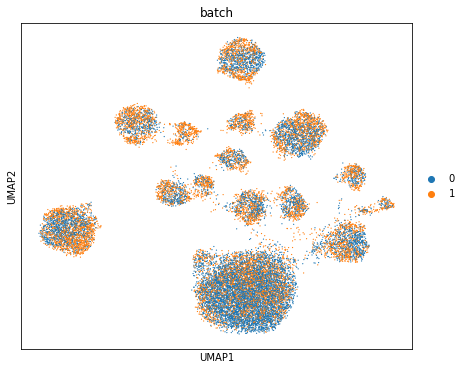
Computing batch mixing

This is a quantitative measure of how well cells mix in the latent space, and is precisely the information entropy of the batch annotations of cells in a given cell’s neighborhood, averaged over the dataset.

full = trainer.create_posterior(trainer.model, retina_dataset, indices=np.arange(len(retina_dataset)))
print("Entropy of batch mixing :", full.entropy_batch_mixing())

Entropy of batch mixing : 0.6212606968643457

Visualizing the mixing

full = trainer.create_posterior(trainer.model, retina_dataset, indices=np.arange(len(retina_dataset)))
latent, batch_indices, labels = full.sequential().get_latent()

post_adata = anndata.AnnData(X=retina_dataset.X)
post_adata.obsm["X_scVI"] = latent
post_adata.obs['cell_type'] = np.array([retina_dataset.cell_types[retina_dataset.labels[i][0]]
                                   for i in range(post_adata.n_obs)])
post_adata.obs['batch'] = np.array([str(retina_dataset.batch_indices[i][0])
                                   for i in range(post_adata.n_obs)])
sc.pp.neighbors(post_adata, use_rep="X_scVI", n_neighbors=15)
sc.tl.umap(post_adata)

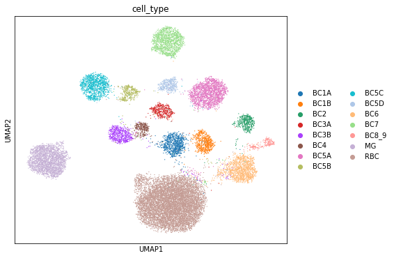
fig, ax = plt.subplots(figsize=(7, 6))
sc.pl.umap(post_adata, color=["cell_type"], ax=ax, show=show_plot)
fig, ax = plt.subplots(figsize=(7, 6))
sc.pl.umap(post_adata, color=["batch"], ax=ax, show=show_plot)

... storing 'cell_type' as categorical
... storing 'batch' as categorical

1.7. Logging information

Verbosity varies in the following way: * logger.setLevel(logging.WARNING) will show a progress bar. * logger.setLevel(logging.INFO) will show global logs including the number of jobs done. * logger.setLevel(logging.DEBUG) will show detailed logs for each training (e.g the parameters tested).

This function’s behaviour can be customized, please refer to its documentation for information about the different parameters available.

In general, you can use scvi.set_verbosity(level) to set the verbosity of the scvi package. Note that level corresponds to the logging levels of the standard python logging module. By default, that level is set to INFO (=20). As a reminder the logging levels are:

Level	Numeric value
CRITICAL	50
ERROR	40
WARNING	30
INFO	20
DEBUG	10
NOTSET	0