ATAC-seq analysis in R

In this tutorial, we go over how to use scvi-tools functionality in R for analyzing ATAC-seq data. We will closely follow the PBMC tutorial from Signac, using scvi-tools when appropriate. In particular, we will

1. Use PeakVI for dimensionality reduction and differential accessiblity for the ATAC-seq data

2. Use scVI to integrate the unpaired ATAC-seq dataset with a match scRNA-seq dataset of PBMCs

This tutorial requires Reticulate. Please check out our installation guide for instructions on installing Reticulate and scvi-tools.

Loading and processing data with Signac

system("wget https://cf.10xgenomics.com/samples/cell-atac/1.0.1/atac_v1_pbmc_10k/atac_v1_pbmc_10k_filtered_peak_bc_matrix.h5")
system("wget https://cf.10xgenomics.com/samples/cell-atac/1.0.1/atac_v1_pbmc_10k/atac_v1_pbmc_10k_singlecell.csv")
system("wget https://cf.10xgenomics.com/samples/cell-atac/1.0.1/atac_v1_pbmc_10k/atac_v1_pbmc_10k_fragments.tsv.gz")
system("wget https://cf.10xgenomics.com/samples/cell-atac/1.0.1/atac_v1_pbmc_10k/atac_v1_pbmc_10k_fragments.tsv.gz.tbi")

library(Signac)
library(Seurat)
library(GenomeInfoDb)
library(EnsDb.Hsapiens.v75)
library(ggplot2)
library(patchwork)
set.seed(1234)

Pre-processing

We follow the original tutorial to create the Seurat object with ATAC data.

counts <- Read10X_h5(filename = "atac_v1_pbmc_10k_filtered_peak_bc_matrix.h5")
metadata <- read.csv(
  file = "atac_v1_pbmc_10k_singlecell.csv",
  header = TRUE,
  row.names = 1
)

chrom_assay <- CreateChromatinAssay(
  counts = counts,
  sep = c(":", "-"),
  genome = 'hg19',
  fragments = 'atac_v1_pbmc_10k_fragments.tsv.gz',
  min.cells = 10,
  min.features = 200
)

pbmc <- CreateSeuratObject(
  counts = chrom_assay,
  assay = "peaks",
  meta.data = metadata
)

pbmc

An object of class Seurat 
87561 features across 8728 samples within 1 assay 
Active assay: peaks (87561 features, 0 variable features)

pbmc[['peaks']]

ChromatinAssay data with 87561 features for 8728 cells
Variable features: 0 
Genome: hg19 
Annotation present: FALSE 
Motifs present: FALSE 
Fragment files: 1 

We add gene annotation information to facilitate downstream functionality.

# extract gene annotations from EnsDb
annotations <- GetGRangesFromEnsDb(ensdb = EnsDb.Hsapiens.v75)

# change to UCSC style since the data was mapped to hg19
seqlevelsStyle(annotations) <- 'UCSC'
genome(annotations) <- "hg19"

# add the gene information to the object
Annotation(pbmc) <- annotations

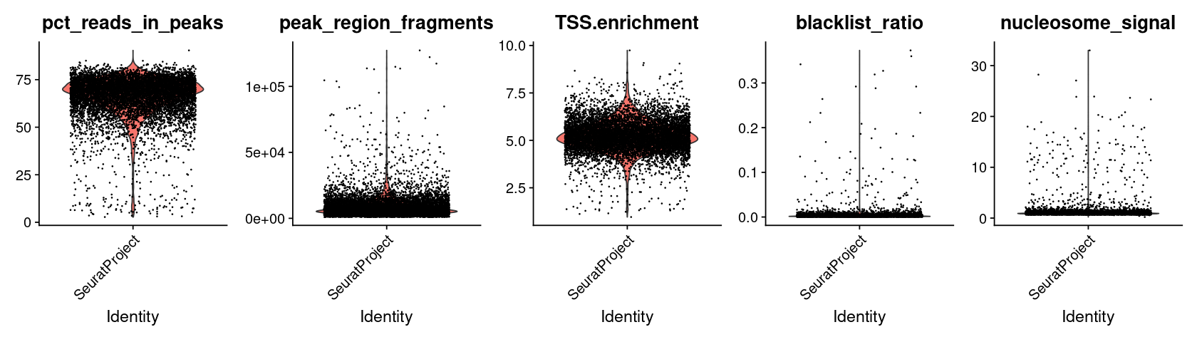
Computing QC metrics

We compute the same QC metrics as the original tutorial. We leave it to the reader to follow the excellent Signac tutorial for understanding what these quantities represent.

# compute nucleosome signal score per cell
pbmc <- NucleosomeSignal(object = pbmc)

# compute TSS enrichment score per cell
pbmc <- TSSEnrichment(object = pbmc, fast = FALSE)

# add blacklist ratio and fraction of reads in peaks
pbmc$pct_reads_in_peaks <- pbmc$peak_region_fragments / pbmc$passed_filters * 100
pbmc$blacklist_ratio <- pbmc$blacklist_region_fragments / pbmc$peak_region_fragments

options(repr.plot.width=14, repr.plot.height=4)
VlnPlot(
  object = pbmc,
  features = c('pct_reads_in_peaks', 'peak_region_fragments',
               'TSS.enrichment', 'blacklist_ratio', 'nucleosome_signal'),
  pt.size = 0.1,
  ncol = 5
)

pbmc <- subset(
  x = pbmc,
  subset = peak_region_fragments > 3000 &
    peak_region_fragments < 20000 &
    pct_reads_in_peaks > 15 &
    blacklist_ratio < 0.05 &
    nucleosome_signal < 4 &
    TSS.enrichment > 2
)
pbmc

An object of class Seurat 
87561 features across 7060 samples within 1 assay 
Active assay: peaks (87561 features, 0 variable features)

Dimensionality reduction (PeakVI)

Creating an AnnData object

We follow the standard workflow for converting between Seurat and AnnData.

library(reticulate)
library(sceasy)
use_python("/home/adam/.pyenv/versions/3.9.7/bin/python", required = TRUE)
sc <- import("scanpy", convert = FALSE)
scvi <- import("scvi", convert = FALSE)

adata <- convertFormat(pbmc, from="seurat", to="anndata", main_layer="counts", assay="peaks", drop_single_values=FALSE)
print(adata) # Note generally in Python, dataset conventions are obs x var

AnnData object with n_obs × n_vars = 7060 × 87561
    obs: 'orig.ident', 'nCount_peaks', 'nFeature_peaks', 'total', 'duplicate', 'chimeric', 'unmapped', 'lowmapq', 'mitochondrial', 'passed_filters', 'cell_id', 'is__cell_barcode', 'TSS_fragments', 'DNase_sensitive_region_fragments', 'enhancer_region_fragments', 'promoter_region_fragments', 'on_target_fragments', 'blacklist_region_fragments', 'peak_region_fragments', 'nucleosome_signal', 'nucleosome_percentile', 'TSS.enrichment', 'TSS.percentile', 'pct_reads_in_peaks', 'blacklist_ratio'
    var: 'count', 'percentile'

Run the standard PeakVI workflow

scvi$model$PEAKVI$setup_anndata(adata)

None

pvi <- scvi$model$PEAKVI(adata)
pvi$train()

None

# get the latent represenation
latent = pvi$get_latent_representation()

# put it back in our original Seurat object
latent <- as.matrix(latent)
rownames(latent) = colnames(pbmc)
ndims <- ncol(latent)
pbmc[["peakvi"]] <- CreateDimReducObject(embeddings = latent, key = "peakvi_", assay = "peaks")

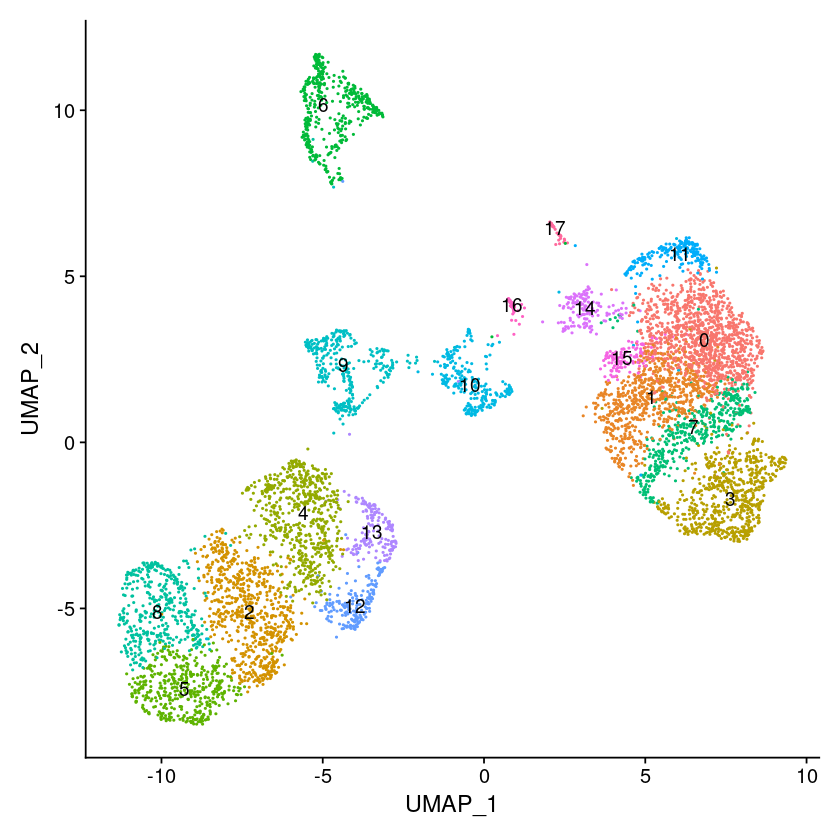
# Find clusters, then run UMAP, and visualize
pbmc <- FindNeighbors(pbmc, reduction = "peakvi", dims=1:ndims)
pbmc <- FindClusters(pbmc, resolution = 1)

pbmc <- RunUMAP(pbmc, reduction = "peakvi", dims=1:ndims)

options(repr.plot.width=7, repr.plot.height=7)
DimPlot(object = pbmc, label = TRUE) + NoLegend()

Modularity Optimizer version 1.3.0 by Ludo Waltman and Nees Jan van Eck

Number of nodes: 7060
Number of edges: 220834

Running Louvain algorithm...
Maximum modularity in 10 random starts: 0.8544
Number of communities: 18
Elapsed time: 0 seconds

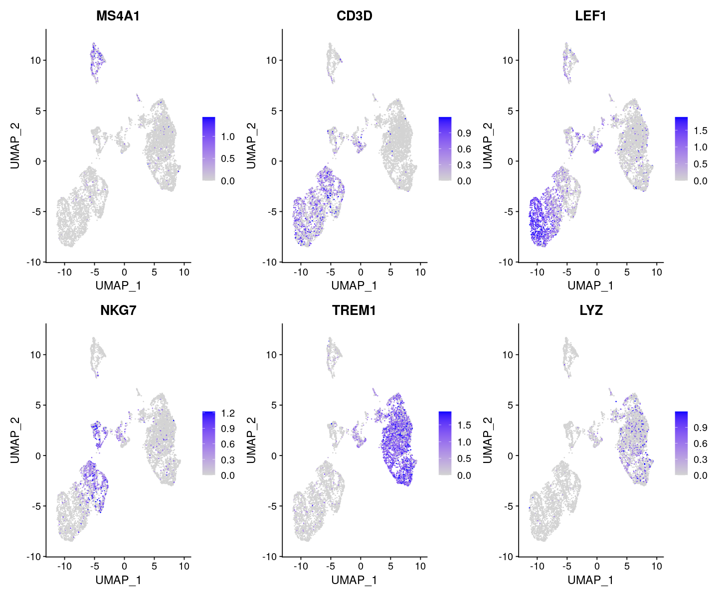
Create a gene activity matrix

Important

The gene activity is used as an approximation of a gene expression matrix such that unpaired ATAC data can be integrated with RNA data. We recommend using this approach only for this unpaired case. Better results can be acheived if there is partially paired data, in which case MultiVI can be used.

gene.activities <- GeneActivity(pbmc)

# add the gene activity matrix to the Seurat object as a new assay and normalize it
pbmc[['RNA']] <- CreateAssayObject(counts = gene.activities)
pbmc <- NormalizeData(
  object = pbmc,
  assay = 'RNA',
  normalization.method = 'LogNormalize',
  scale.factor = median(pbmc$nCount_RNA)
)

options(repr.plot.width=12, repr.plot.height=10)

DefaultAssay(pbmc) <- 'RNA'

FeaturePlot(
  object = pbmc,
  features = c('MS4A1', 'CD3D', 'LEF1', 'NKG7', 'TREM1', 'LYZ'),
  pt.size = 0.1,
  max.cutoff = 'q95',
  ncol = 3
)

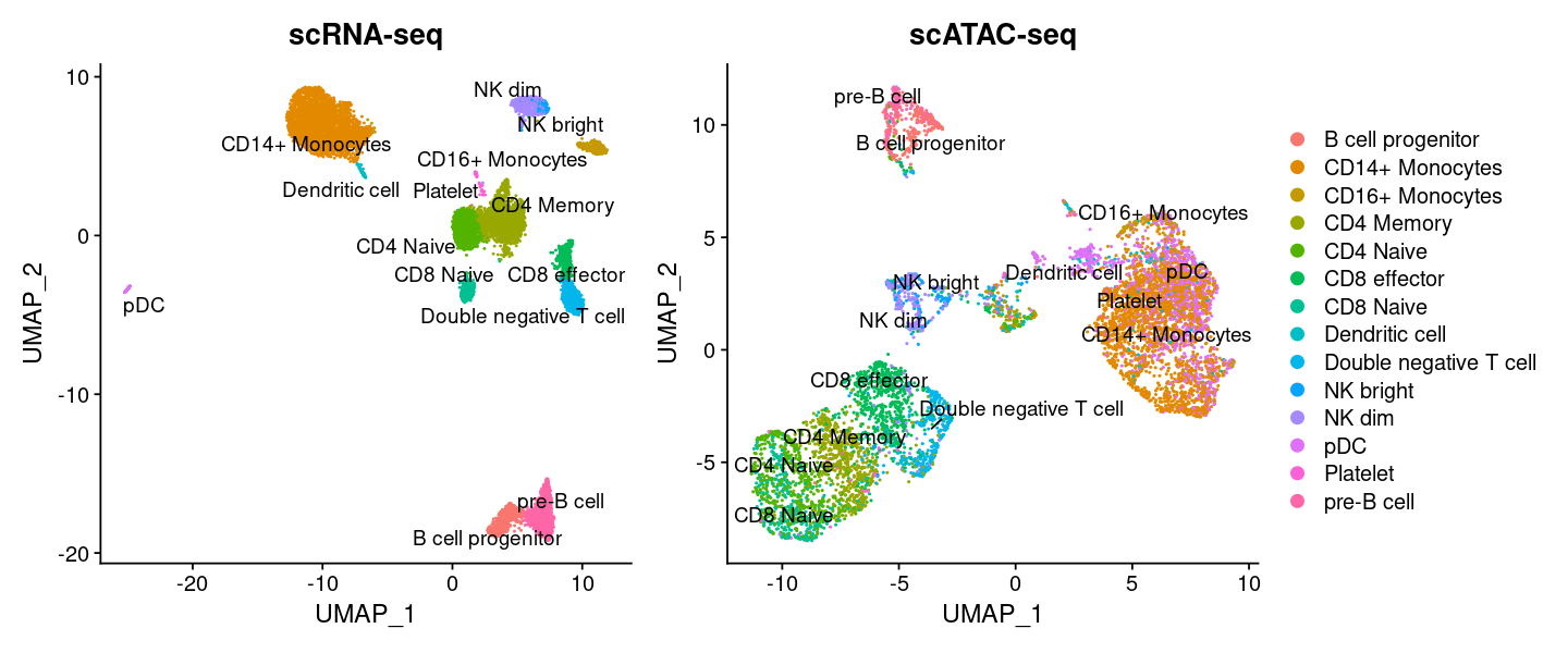
Integrating with scRNA-seq data (scANVI)

We can integrate the gene activity matrix with annotated scRNA-seq data using scANVI.

First we download the Seurat-processed PBMC 10k dataset (as in their tutorial).

system("wget https://www.dropbox.com/s/zn6khirjafoyyxl/pbmc_10k_v3.rds?dl=1 -O pbmc_10k_v3.rds")

pbmc_rna <- readRDS("pbmc_10k_v3.rds")

And we convert it to AnnData using sceasy again. Subsequently, we follow the standard scANVI workflow: pretraining with scVI then running scANVI.

adata_rna <- convertFormat(pbmc_rna, from="seurat", to="anndata", main_layer="counts", assay="RNA", drop_single_values=FALSE)
adata_atac_act <- convertFormat(pbmc, from="seurat", to="anndata", main_layer="counts", assay="RNA", drop_single_values=FALSE)

# provide adata_atac_act unknown cell type labels
adata_atac_act$obs$insert(adata_atac_act$obs$shape[1], "celltype", "Unknown")

adata_both <- adata_rna$concatenate(adata_atac_act)

None

We concatenated the RNA expression with the activity matrix using AnnData. Now we can see the last column is called “batch” and denotes which dataset each cell originated from.

head(py_to_r(adata_both$obs))

A data.frame: 6 × 35

	orig.ident	nCount_RNA	nFeature_RNA	observed	simulated	percent.mito	RNA_snn_res.0.4	celltype	nCount_peaks	nFeature_peaks	⋯	peak_region_fragments	nucleosome_signal	nucleosome_percentile	TSS.enrichment	TSS.percentile	pct_reads_in_peaks	blacklist_ratio	peaks_snn_res.1	seurat_clusters	batch
	<chr>	<dbl>	<int>	<dbl>	<dbl>	<dbl>	<fct>	<chr>	<dbl>	<dbl>	⋯	<dbl>	<dbl>	<dbl>	<dbl>	<dbl>	<dbl>	<dbl>	<fct>	<fct>	<fct>
rna_AAACCCAAGCGCCCAT-1-0	10x_RNA	2204	1087	0.035812672	0.4382022	0.02359347	1	CD4 Memory	NaN	NaN	⋯	NaN	NaN	NaN	NaN	NaN	NaN	NaN	NA	NA	0
rna_AAACCCACAGAGTTGG-1-0	10x_RNA	5884	1836	0.019227034	0.1017964	0.10757988	0	CD14+ Monocytes	NaN	NaN	⋯	NaN	NaN	NaN	NaN	NaN	NaN	NaN	NA	NA	0
rna_AAACCCACAGGTATGG-1-0	10x_RNA	5530	2216	0.005447865	0.1392801	0.07848101	5	NK dim	NaN	NaN	⋯	NaN	NaN	NaN	NaN	NaN	NaN	NaN	NA	NA	0
rna_AAACCCACATAGTCAC-1-0	10x_RNA	5106	1615	0.014276003	0.4949495	0.10830396	3	pre-B cell	NaN	NaN	⋯	NaN	NaN	NaN	NaN	NaN	NaN	NaN	NA	NA	0
rna_AAACCCACATCCAATG-1-0	10x_RNA	4572	1800	0.053857351	0.1392801	0.08989501	5	NK bright	NaN	NaN	⋯	NaN	NaN	NaN	NaN	NaN	NaN	NaN	NA	NA	0
rna_AAACCCAGTGGCTACC-1-0	10x_RNA	6702	1965	0.056603774	0.3554328	0.06326470	1	CD4 Memory	NaN	NaN	⋯	NaN	NaN	NaN	NaN	NaN	NaN	NaN	NA	NA	0

sc$pp$highly_variable_genes(
    adata_both, 
    flavor="seurat_v3", 
    n_top_genes=r_to_py(3000), 
    batch_key="batch", 
    subset=TRUE
)
scvi$model$SCVI$setup_anndata(adata_both, labels_key="celltype", batch_key="batch")

None

None

model <- scvi$model$SCVI(adata_both, gene_likelihood="nb", dispersion="gene-batch")
model$train()

None

lvae <- scvi$model$SCANVI$from_scvi_model(model, "Unknown", adata=adata_both)
lvae$train(max_epochs = as.integer(100), n_samples_per_label = as.integer(100))

None

Here we only use the prediction functionality of scANVI, but we also could have viewed an integrated representation of the ATAC and RNA using UMAP.

adata_both$obs$insert(adata_both$obs$shape[1], "predicted.labels", lvae$predict())
df <- py_to_r(adata_both$obs)
df <- subset(df, batch == 1)[, c("predicted.labels")]
pbmc <- AddMetaData(object = pbmc, metadata = df, col.name="predicted.labels")

None

Important

These labels should only serve as a starting point. Further inspection should always be performed. We leave this to the user, but will continue with these labels as a demonstration.

options(repr.plot.width=12, repr.plot.height=5)

plot1 <- DimPlot(
  object = pbmc_rna,
  group.by = 'celltype',
  label = TRUE,
  repel = TRUE) + NoLegend() + ggtitle('scRNA-seq')

plot2 <- DimPlot(
  object = pbmc,
  group.by = 'predicted.labels',
  label = TRUE,
  repel = TRUE) + ggtitle('scATAC-seq')

plot1 + plot2

Finding differentially accessible peaks between clusters

As PeakVI learns uncertainty around the observed data, it can be leveraged for differential accessibility analysis. First, let’s store the seurat cluster information back inside the AnnData.

adata$obs$insert(adata$obs$shape[1], "predicted_ct", pbmc[["predicted.labels"]][,1])

None

Using our trained PEAKVI model, we call the differential_accessibility() (DA) method We pass predicted_ct to the groupby argument and compare between naive CD4s and CD14 monocytes.

The output of DA is a DataFrame with the bayes factors. Bayes factors > 3 have high probability of being differentially expressed. You can also set fdr_target, which will return the differentially expressed genes based on the posteior expected FDR.

DA <- pvi$differential_accessibility(adata, groupby="predicted_ct", group1 = "CD4 Naive", group2 = "CD14+ Monocytes")
DA <- py_to_r(DA)
head(DA)

A data.frame: 6 × 9

	prob_da	is_da_fdr	bayes_factor	effect_size	emp_effect	est_prob1	est_prob2	emp_prob1	emp_prob2
	<dbl>	<lgl>	<dbl>	<dbl>	<dbl>	<dbl>	<dbl>	<dbl>	<dbl>
chr1-565107-565550	0.0738	FALSE	-2.5297313	-0.02128995	-0.009461094	0.03177977	0.010489821	0.014539580	0.005078486
chr1-569174-569639	0.5342	FALSE	0.1370139	-0.06247292	-0.026307585	0.08119156	0.018718639	0.035541195	0.009233610
chr1-713460-714823	0.9208	TRUE	2.4532664	-0.27283466	-0.164037549	0.73534369	0.462509036	0.389337641	0.225300092
chr1-752422-753038	0.9722	TRUE	3.5545252	0.18390924	0.093491423	0.01899158	0.202900812	0.004846527	0.098337950
chr1-762106-763359	0.8202	FALSE	1.5177030	-0.15394741	-0.096660536	0.51465970	0.360712290	0.266558966	0.169898430
chr1-779589-780271	0.7834	FALSE	1.2855911	-0.09098869	-0.049387882	0.09661592	0.005627228	0.051696284	0.002308403

# sort by proba_da and effect_size
DA <- DA[order(-DA[, 1], -DA[, 4]), ]
head(DA)

A data.frame: 6 × 9

	prob_da	is_da_fdr	bayes_factor	effect_size	emp_effect	est_prob1	est_prob2	emp_prob1	emp_prob2
	<dbl>	<lgl>	<dbl>	<dbl>	<dbl>	<dbl>	<dbl>	<dbl>	<dbl>
chr17-1510080-1511616	1.0000	TRUE	18.420681	0.8669005	0.4471439	0.04267091	0.90957141	0.027463651	0.474607572
chr8-141108218-141111251	1.0000	TRUE	18.420681	-0.8540915	-0.4437980	0.89332950	0.03923802	0.466882068	0.023084026
chr14-50504661-50507777	0.9998	TRUE	8.516943	0.8495569	0.5436486	0.14001995	0.98957688	0.085621971	0.629270545
chr19-36397851-36401040	0.9998	TRUE	8.516943	0.8030195	0.3956684	0.07268646	0.87570596	0.035541195	0.431209603
chr7-6674416-6675306	0.9998	TRUE	8.516943	0.4002175	0.1814427	0.01607980	0.41629726	0.009693053	0.191135734
chr1-23945628-23947309	0.9998	TRUE	8.516943	-0.7074655	-0.3593336	0.72208506	0.01461957	0.366720517	0.007386888

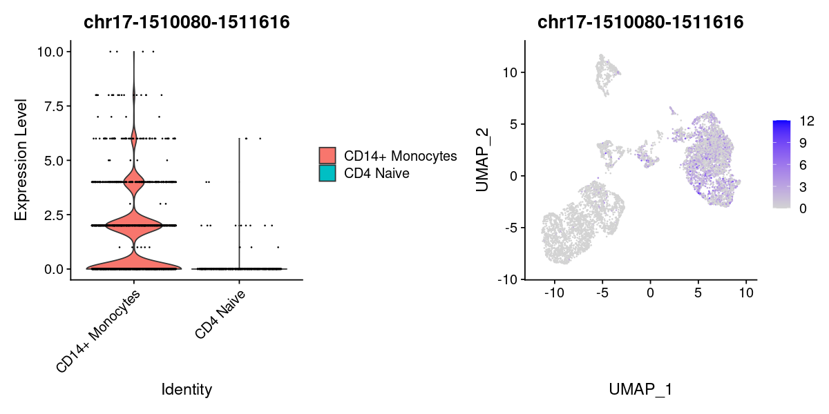
options(repr.plot.width=10, repr.plot.height=5)

DefaultAssay(pbmc) <- 'peaks'
Idents(pbmc) <- pbmc[["predicted.labels"]]

plot1 <- VlnPlot(
  object = pbmc,
  features = rownames(DA)[1],
  pt.size = 0.1,
  idents = c("CD4 Naive","CD14+ Monocytes")
)
plot2 <- FeaturePlot(
  object = pbmc,
  features = rownames(DA)[1],
  pt.size = 0.1
)

plot1 | plot2

sI <- sessionInfo()
sI$loadedOnly <- NULL
print(sI, locale=FALSE)

R version 4.1.0 (2021-05-18)
Platform: x86_64-pc-linux-gnu (64-bit)
Running under: Ubuntu 20.04.2 LTS

Matrix products: default
BLAS:   /usr/lib/x86_64-linux-gnu/blas/libblas.so.3.9.0
LAPACK: /usr/lib/x86_64-linux-gnu/lapack/liblapack.so.3.9.0

attached base packages:
[1] stats4    stats     graphics  grDevices utils     datasets  methods  
[8] base     

other attached packages:
 [1] sceasy_0.0.6              reticulate_1.20          
 [3] patchwork_1.1.1           ggplot2_3.3.5            
 [5] EnsDb.Hsapiens.v75_2.99.0 ensembldb_2.17.4         
 [7] AnnotationFilter_1.17.1   GenomicFeatures_1.45.2   
 [9] AnnotationDbi_1.55.1      Biobase_2.53.0           
[11] GenomicRanges_1.45.0      GenomeInfoDb_1.29.8      
[13] IRanges_2.27.2            S4Vectors_0.31.3         
[15] BiocGenerics_0.39.2       SeuratObject_4.0.2       
[17] Seurat_4.0.4              Signac_1.3.0