Multi-resolution deconvolution of spatial transcriptomics

In this tutorial, we through the steps of applying DestVI for deconvolution of 10x Visium spatial transcriptomics profiles using an accompanying single-cell RNA sequencing data.

Background:

Spatial transcriptomics technologies are currently limited, because their resolution is limited to niches (spots) of sizes well beyond that of a single cell. Although several pipelines proposed joint analysis with single-cell RNA-sequencing (scRNA-seq) to alleviate this problem they are limited to a discrete view of cell type proportion inside every spot. This limitation becomes critical in the common case where, even within a cell type, there is a continuum of cell states. We present Deconvolution of Spatial Transcriptomics profiles using Variational Inference (DestVI), a probabilistic method for multi-resolution analysis for spatial transcriptomics that explicitly models continuous variation within cell types.

Plan for this tutorial:

1. Loading the data

2. Training the single-cell model (scLVM) to learn a basis of gene expression on the scRNA-seq data

3. Training the spatial model (stLVM) to perform the deconvolution

4. Visualize the learned cell type proportions

5. Run our automated pipeline

6. Dig into the intra cell type information

7. Run cell-type specific differential expression

Note

Running the following cell will install tutorial dependencies on Google Colab only. It will have no effect on environments other than Google Colab.

!pip install --quiet scvi-colab
from scvi_colab import install

install()
!pip install --quiet git+https://github.com/yoseflab/destvi_utils.git@main

import tempfile

import destvi_utils
import matplotlib.pyplot as plt
import numpy as np
import scanpy as sc
import scvi
import seaborn as sns
import torch
from scvi.model import CondSCVI, DestVI

scvi.settings.seed = 0
print("Last run with scvi-tools version:", scvi.__version__)

Last run with scvi-tools version: 1.4.0.post1

Note

You can modify save_dir below to change where the data files for this tutorial are saved.

sc.set_figure_params(figsize=(6, 6), frameon=False)
sns.set_theme()
torch.set_float32_matmul_precision("high")
save_dir = tempfile.TemporaryDirectory()

%config InlineBackend.print_figure_kwargs={"facecolor": "w"}
%config InlineBackend.figure_format="retina"

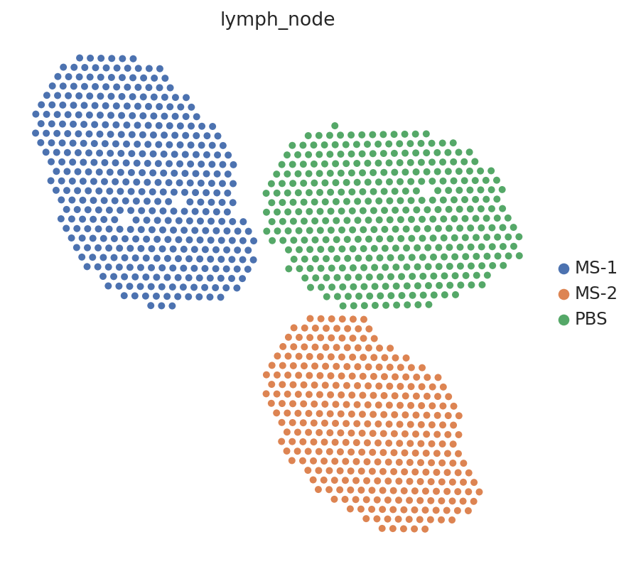
Let’s download our data from a comparative study of murine lymph nodes, comparing wild-type with a stimulation after injection of a mycobacteria. We have at disposal a 10x Visium dataset as well as a matching scRNA-seq dataset from the same tissue.

url1 = "https://github.com/romain-lopez/DestVI-reproducibility/blob/master/lymph_node/deconvolution/ST-LN-compressed.h5ad?raw=true"
url2 = "https://github.com/romain-lopez/DestVI-reproducibility/blob/master/lymph_node/deconvolution/scRNA-LN-compressed.h5ad?raw=true"
out1 = "data/ST-LN-compressed.h5ad"
out2 = "data/scRNA-LN-compressed.h5ad"

Data loading & processing

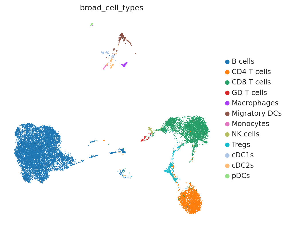
First, let’s load the single-cell data. We profiled immune cells from murine lymph nodes with 10x Chromium, as a control / case study to study the immune response to exposure to a mycobacteria (refer to our paper for more info). We provide the preprocessed data from our reproducibility repository: it contains the raw counts (DestVI always takes raw counts as input).

sc_adata = sc.read(out2, backup_url=url2)

We clustered the single-cell data by major immune cell types. DestVI can resolve beyond discrete clusters, but need to work with an existing level of clustering. A rule of thumb to keep in mind while clsutering is that DestVI assumes only a single state from each cell type exists in each spot. For example, resting and inflammed monocytes cannot co-exist in one unique spot according to our assumption. Users may cluster their data so that this modeling assumption is as accurate as possible.

sc.pl.umap(sc_adata, color="broad_cell_types")

# let us filter some genes
G = 2000
sc.pp.filter_genes(sc_adata, min_counts=10)

sc_adata.layers["counts"] = sc_adata.X.copy()

sc.pp.highly_variable_genes(
    sc_adata, n_top_genes=G, subset=True, layer="counts", flavor="seurat_v3"
)

sc.pp.normalize_total(sc_adata, target_sum=10e4)
sc.pp.log1p(sc_adata)
sc_adata.raw = sc_adata

Now, let’s load the spatial data and choose a common gene subset. Users will note that having a common gene set is a prerequisite of the method.

st_adata = sc.read(out1, backup_url=url1)

st_adata.layers["counts"] = st_adata.X.copy()
st_adata.obsm["spatial"] = st_adata.obsm["location"]

sc.pp.normalize_total(st_adata, target_sum=10e4)
sc.pp.log1p(st_adata)
st_adata.raw = st_adata

# filter genes to be the same on the spatial data
intersect = np.intersect1d(sc_adata.var_names, st_adata.var_names)
st_adata = st_adata[:, intersect].copy()
sc_adata = sc_adata[:, intersect].copy()
G = len(intersect)

sc.pl.embedding(st_adata, basis="spatial", color="lymph_node", s=80)

Fit the scLVM

In order to learn cell state specific gene expression patterns, we will fit the single-cell Latent Variable Model (scLVM) to single-cell RNA sequencing data from the same tissue.

sc_adata.obs.head()

	n_genes	cell_types	batch	n_genes_by_counts	total_counts	total_counts_mt	pct_counts_mt	pred_cell_types	doublet_scores	doublet_predictions	...	louvain_sub_0.1	louvain_sub_0.2	louvain_sub_0.3	louvain_sub	louvain_sub_1	louvain_sub_2	louvain_sub_3	SCANVI_pred_cell_types	SCVI_pred_cell_types	broad_cell_types
AAACCCAAGCAGAAAG-1-0	1505	Tregs	0	1505	5862.0	307.0	5.237121	Tregs	0.090909	0.0	...	6	6	6	Tregs	Tregs	6,1	6,1	Tregs	Tregs	Tregs
AAACCCAAGGTCACAG-1-0	1883	Mature B cells	0	1883	6673.0	346.0	5.185074	Mature B	0.116751	0.0	...	0	0	0	B cells,0	B cells,0	0	0	Cycling B/T cells	Mature B	B cells
AAACCCACATCGTTCC-1-0	2080	CD8 T cells	0	2080	7764.0	438.0	5.641422	CD122+ CD8 T	0.041626	0.0	...	1	1-3,0	1	CD8 T cells	CD8 T cells	1-3,0	1-3,0	CD8 T	CD8 T	CD8 T cells
AAACCCAGTCGTCTCT-1-0	1647	Cycling B/T cells	0	1647	4619.0	265.0	5.737173	Mature B	0.098634	0.0	...	5	5	5	B cells,7	B cells,7	5	5	Ifit3-high B	Mature B	B cells
AAACCCAGTGTAAACA-1-0	1857	Mature B cells	0	1857	5965.0	339.0	5.683152	Mature B	0.153374	0.0	...	0	0	0	B cells,3	B cells,3	0	0	B-macrophage doublets	Mature B	B cells

5 rows × 31 columns

CondSCVI.setup_anndata(
    sc_adata,
    layer="counts",
    labels_key="broad_cell_types",
    fine_labels_key="cell_types",
    batch_key="batch",
)

As a first step, we embed our data using a cell type conditional VAE. We pass the layer containing the raw counts and the labels key. We train this model without reweighting the loss by the cell type abundance. Training will take around 5 minutes in a Colab GPU session.

sc_model = CondSCVI(sc_adata, weight_obs=False, prior="mog", num_classes_mog=10)
sc_model.view_anndata_setup()

Anndata setup with scvi-tools version 1.4.0.post1.

Setup via `CondSCVI.setup_anndata` with arguments:

{
│   'batch_key': 'batch',
│   'labels_key': 'broad_cell_types',
│   'fine_labels_key': 'cell_types',
│   'layer': 'counts',
│   'unlabeled_category': 'unlabeled',
│   'size_factor_key': None
}

     Summary Statistics     
┏━━━━━━━━━━━━━━━━━━┳━━━━━━━┓
┃ Summary Stat Key ┃ Value ┃
┡━━━━━━━━━━━━━━━━━━╇━━━━━━━┩
│     n_batch      │   4   │
│     n_cells      │ 14989 │
│  n_fine_labels   │  16   │
│     n_labels     │  12   │
│      n_vars      │ 1888  │
└──────────────────┴───────┘

                  Data Registry                  
┏━━━━━━━━━━━━━━┳━━━━━━━━━━━━━━━━━━━━━━━━━━━━━━━━┓
┃ Registry Key ┃      scvi-tools Location       ┃
┡━━━━━━━━━━━━━━╇━━━━━━━━━━━━━━━━━━━━━━━━━━━━━━━━┩
│      X       │     adata.layers['counts']     │
│    batch     │    adata.obs['_scvi_batch']    │
│ fine_labels  │ adata.obs['_scvi_fine_labels'] │
│    labels    │   adata.obs['_scvi_labels']    │
└──────────────┴────────────────────────────────┘

                         labels State Registry                         
┏━━━━━━━━━━━━━━━━━━━━━━━━━━━━━━━┳━━━━━━━━━━━━━━━┳━━━━━━━━━━━━━━━━━━━━━┓
┃        Source Location        ┃  Categories   ┃ scvi-tools Encoding ┃
┡━━━━━━━━━━━━━━━━━━━━━━━━━━━━━━━╇━━━━━━━━━━━━━━━╇━━━━━━━━━━━━━━━━━━━━━┩
│ adata.obs['broad_cell_types'] │    B cells    │          0          │
│                               │  CD4 T cells  │          1          │
│                               │  CD8 T cells  │          2          │
│                               │  GD T cells   │          3          │
│                               │  Macrophages  │          4          │
│                               │ Migratory DCs │          5          │
│                               │   Monocytes   │          6          │
│                               │   NK cells    │          7          │
│                               │     Tregs     │          8          │
│                               │     cDC1s     │          9          │
│                               │     cDC2s     │         10          │
│                               │     pDCs      │         11          │
└───────────────────────────────┴───────────────┴─────────────────────┘

                  batch State Registry                   
┏━━━━━━━━━━━━━━━━━━━━┳━━━━━━━━━━━━┳━━━━━━━━━━━━━━━━━━━━━┓
┃  Source Location   ┃ Categories ┃ scvi-tools Encoding ┃
┡━━━━━━━━━━━━━━━━━━━━╇━━━━━━━━━━━━╇━━━━━━━━━━━━━━━━━━━━━┩
│ adata.obs['batch'] │     0      │          0          │
│                    │     1      │          1          │
│                    │     2      │          2          │
│                    │     3      │          3          │
└────────────────────┴────────────┴─────────────────────┘

                       fine_labels State Registry                       
┏━━━━━━━━━━━━━━━━━━━━━━━━━┳━━━━━━━━━━━━━━━━━━━━━━┳━━━━━━━━━━━━━━━━━━━━━┓
┃     Source Location     ┃      Categories      ┃ scvi-tools Encoding ┃
┡━━━━━━━━━━━━━━━━━━━━━━━━━╇━━━━━━━━━━━━━━━━━━━━━━╇━━━━━━━━━━━━━━━━━━━━━┩
│ adata.obs['cell_types'] │     CD4 T cells      │          0          │
│                         │     CD8 T cells      │          1          │
│                         │ Cxcl9-high monocytes │          2          │
│                         │  Cycling B/T cells   │          3          │
│                         │      GD T cells      │          4          │
│                         │  Ifit3-high B cells  │          5          │
│                         │  Ly6-high monocytes  │          6          │
│                         │     Macrophages      │          7          │
│                         │    Mature B cells    │          8          │
│                         │    Migratory DCs     │          9          │
│                         │       NK cells       │         10          │
│                         │        Tregs         │         11          │
│                         │        cDC1s         │         12          │
│                         │        cDC2s         │         13          │
│                         │         pDCs         │         14          │
│                         │      unlabeled       │         15          │
└─────────────────────────┴──────────────────────┴─────────────────────┘

sc_model.train()

sc_model.history["elbo_train"].iloc[5:].plot()
plt.show()

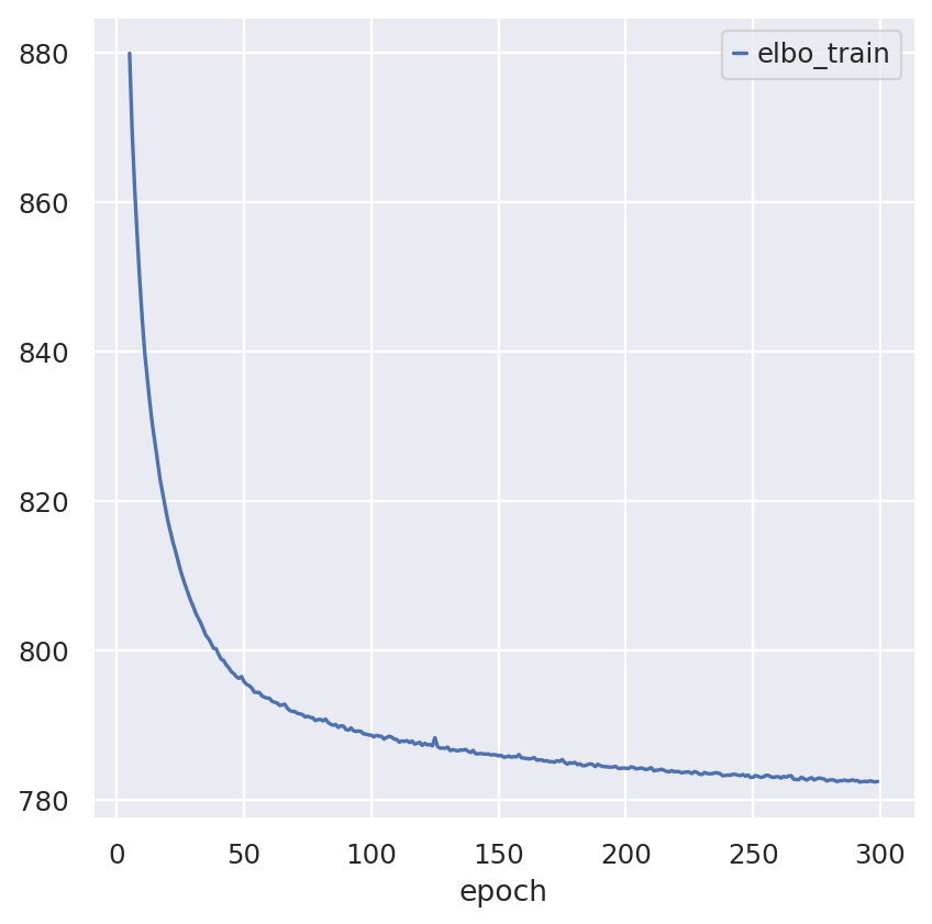
Note that model converges quickly. Over experimentation with the model drastically reducing the number of epochs leads to decreased performance and performance deteriorates as max_epochs<200.

Deconvolution with stLVM

As a second step, we train our deconvolution model: spatial transcriptomics Latent Variable Model (stLVM). We setup the DestVI model using the counts layer in st_adata that contains the raw counts. We then pass the trained CondSCVI model and generate a new model based on st_adata and sc_model using DestVI.from_rna_model.

# Deconvolution with stLVM
st_adata = st_adata[st_adata.layers["counts"].sum(1) > 10].copy()
st_adata.obs["batch"] = "spatial"


def spatial_nn_gex_smth(stadata, n_neighs):
    sc.pp.neighbors(stadata, n_neighs, use_rep="spatial", key_added="Xspatial")
    stadata.obsp["Xspatial_connectivities"] = stadata.obsp["Xspatial_connectivities"].ceil()
    stadata.obsp["Xspatial_connectivities"].setdiag(1)
    return stadata.obsp["Xspatial_connectivities"].dot(stadata.layers["counts"])


st_adata.layers["smoothed"] = spatial_nn_gex_smth(st_adata, n_neighs=5)

The decoder network architecture will be generated from sc_model. Two neural networks are initiated for cell type proportions and gamma value amortization. Training will take around 5 minutes in a Colab GPU session.

Potential adaptations of DestVI.from_rna_model are:

1. increasing vamp_prior_p leads to less gradual changes in gamma values

2. more discretized values. Increasing l1_sparsity will lead to sparser results for cell type proportions.

3. Although we recommend using similar sequencing technology for both assays, consider changing beta_weighting_prior otherwise.

Technical Note: During inference, we adopt a variational mixture of posterior as a prior to enforce gamma values in stLVM match scLVM (see details in original publication). This empirical prior is based on cell type specific subclustering (using k-means to find vamp_prior_p clusters) of the posterior distribution in latent space for every cell.

st_model = DestVI.from_rna_model(
    st_adata,
    sc_model,
    add_celltypes=2,
    n_latent_amortization=None,
    anndata_setup_kwargs={"smoothed_layer": "smoothed"},
)
st_model.view_anndata_setup()

Anndata setup with scvi-tools version 1.4.0.post1.

Setup via `DestVI.setup_anndata` with arguments:

{'layer': 'counts', 'smoothed_layer': 'smoothed', 'batch_key': 'batch'}

     Summary Statistics     
┏━━━━━━━━━━━━━━━━━━┳━━━━━━━┓
┃ Summary Stat Key ┃ Value ┃
┡━━━━━━━━━━━━━━━━━━╇━━━━━━━┩
│     n_batch      │   5   │
│     n_cells      │ 1092  │
│      n_vars      │ 1888  │
│   n_x_smoothed   │ 1888  │
└──────────────────┴───────┘

               Data Registry               
┏━━━━━━━━━━━━━━┳━━━━━━━━━━━━━━━━━━━━━━━━━━┓
┃ Registry Key ┃   scvi-tools Location    ┃
┡━━━━━━━━━━━━━━╇━━━━━━━━━━━━━━━━━━━━━━━━━━┩
│      X       │  adata.layers['counts']  │
│    batch     │ adata.obs['_scvi_batch'] │
│    ind_x     │  adata.obs['_indices']   │
│  x_smoothed  │ adata.layers['smoothed'] │
└──────────────┴──────────────────────────┘

                  batch State Registry                   
┏━━━━━━━━━━━━━━━━━━━━┳━━━━━━━━━━━━┳━━━━━━━━━━━━━━━━━━━━━┓
┃  Source Location   ┃ Categories ┃ scvi-tools Encoding ┃
┡━━━━━━━━━━━━━━━━━━━━╇━━━━━━━━━━━━╇━━━━━━━━━━━━━━━━━━━━━┩
│ adata.obs['batch'] │     0      │          0          │
│                    │     1      │          1          │
│                    │     2      │          2          │
│                    │     3      │          3          │
│                    │  spatial   │          4          │
└────────────────────┴────────────┴─────────────────────┘

st_model.train(max_epochs=2500)

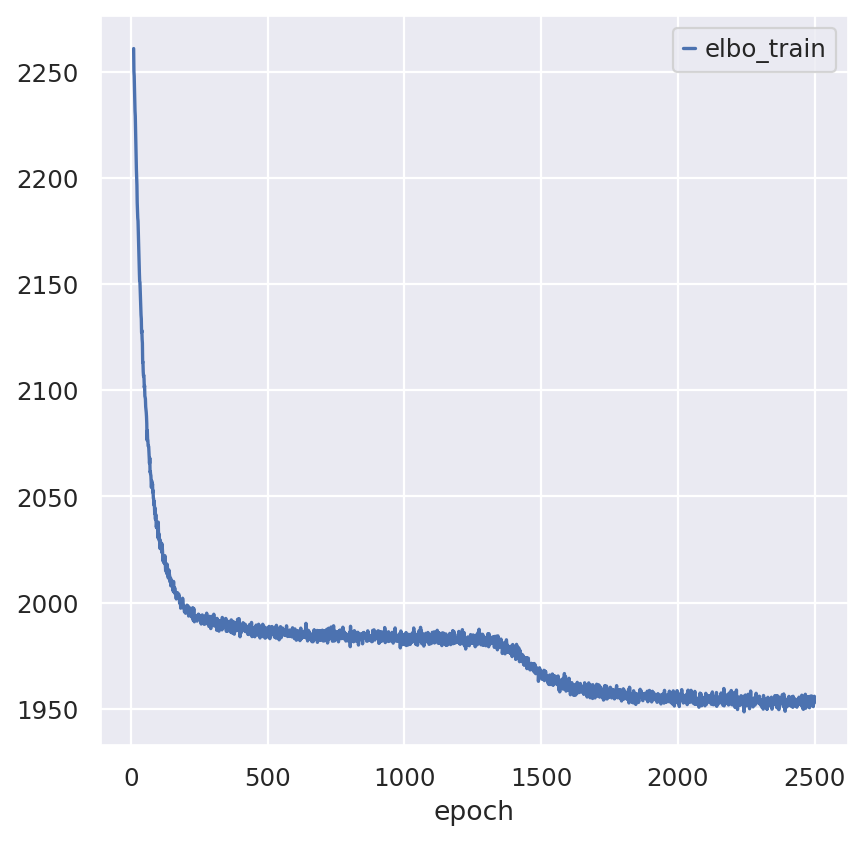
Note that model converges quickly. Over experimentation with the model drastically reducing the number of epochs leads to decreased performance and we advocate against max_epochs<1000.

st_model.history["elbo_train"].iloc[10:].plot()
plt.show()

The output of DestVI has two resolution. At the broader resolution, DestVI returns the cell type proportion in every spot. At the more granular resolution, DestVI can impute cell type specific gene expression in every spot.

Cell type proportions

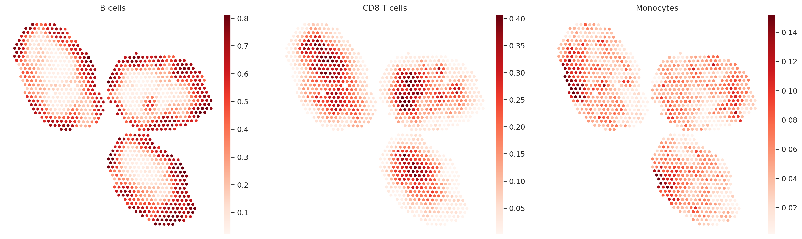
We extract the computed cell type proportions and display them in spatial embedding. These values are directly calculated by normalized the spot-level parameters from the stLVM model.

st_adata.obsm["proportions"] = st_model.get_proportions()

st_adata.obsm["proportions"].head(5)

	B cells	CD4 T cells	CD8 T cells	GD T cells	Macrophages	Migratory DCs	Monocytes	NK cells	Tregs	cDC1s	cDC2s	pDCs
AAACCGGGTAGGTACC-1-0	0.614641	0.006973	0.098060	0.008689	0.048782	0.025055	0.063510	0.000983	0.035803	0.068723	0.014580	0.014202
AAACCTCATGAAGTTG-1-0	0.624894	0.032680	0.036796	0.027864	0.027050	0.051196	0.048278	0.001305	0.080490	0.053341	0.011157	0.004949
AAAGACTGGGCGCTTT-1-0	0.579505	0.035993	0.072657	0.009243	0.043479	0.072511	0.016074	0.003305	0.082376	0.054332	0.021667	0.008858
AAAGGGCAGCTTGAAT-1-0	0.132107	0.051987	0.341011	0.036049	0.057761	0.136065	0.052625	0.006519	0.122469	0.047471	0.010136	0.005799
AAAGTCGACCCTCAGT-1-0	0.800040	0.031249	0.003172	0.023120	0.040634	0.016293	0.020085	0.001624	0.014471	0.044327	0.003878	0.001108

ct_list = ["B cells", "CD8 T cells", "Monocytes"]
for ct in ct_list:
    data = st_adata.obsm["proportions"][ct].values
    st_adata.obs[ct] = np.clip(data, 0, np.quantile(data, 0.99))

sc.pl.embedding(st_adata, basis="spatial", color=ct_list, cmap="Reds", s=80)

Because the inference of cell type specific gene expression is prone to error when the cell type is not present in a spot, and because the cell type proportion values estimated by stLVM are not sparse, we provide an automated way of thresholding them. For follow-up analysis we recommend checking these threshold values and adjust them for each cell type.

This part of the software is not directly available in scvi-tools, but instead in the util package destvi_utils (installable from GitHub; refer to the top of this tutorial).

ct_thresholds = destvi_utils.automatic_proportion_threshold(
    st_adata, ct_list=ct_list, kind_threshold="secondary"
)

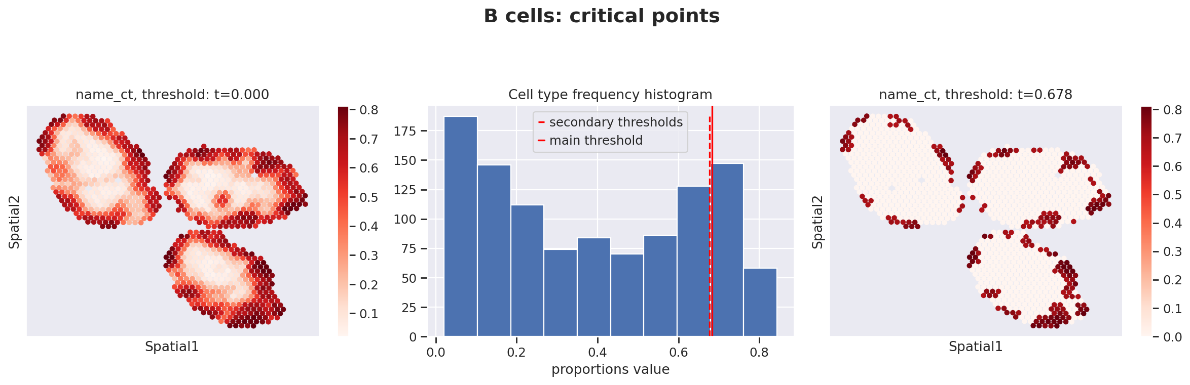
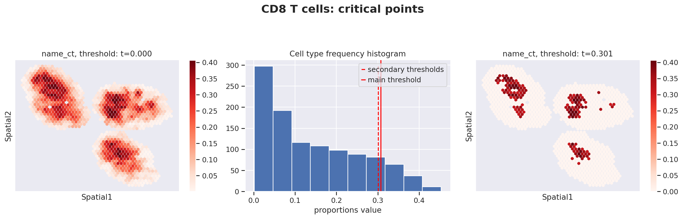
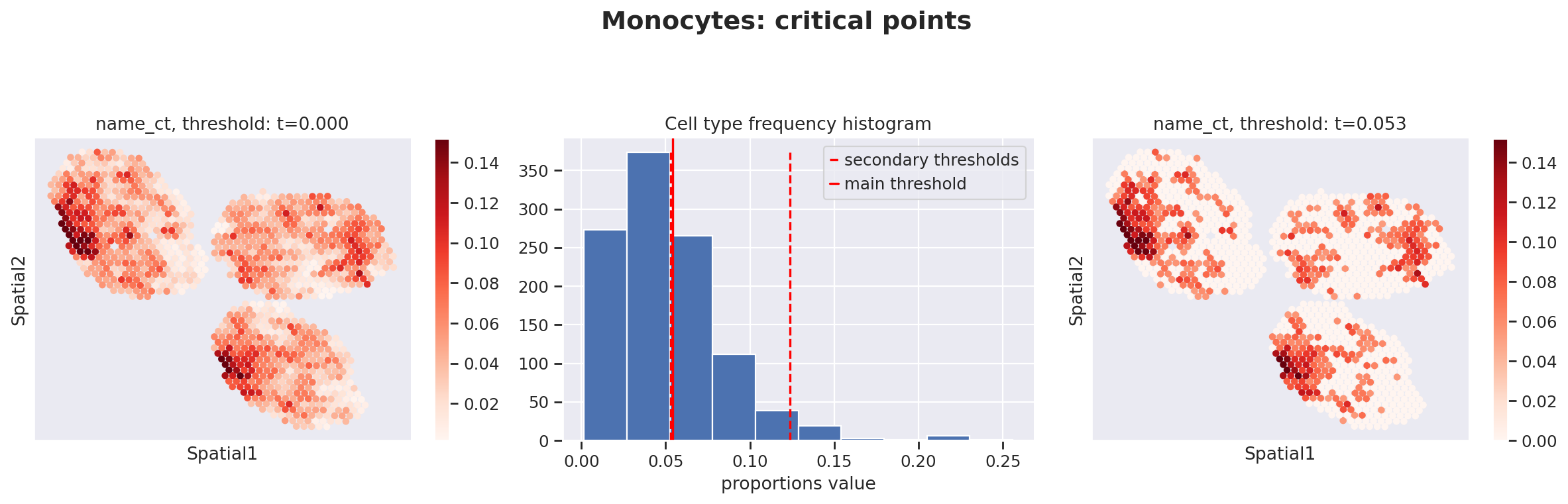
In terms of cell type location, we observe a strong compartimentalization of the cell types in the lymph node (B cells / T cells), as expected. We also observe a differential localization of the monocytes (refer to the paper for further details).

Intra cell type information

At the heart of DestVI is a multitude of latent variables (5 per cell type per spots). We refer to them as “gamma”, and we may manually examine them for downstream analysis

# more globally, the values of the gamma are all summarized in this dictionary of data frames
for ct, g in st_model.get_gamma().items():
    st_adata.obsm[f"{ct}_gamma"] = g

st_adata.obsm["B cells_gamma"].head(5)

	0	1	2	3	4
AAACCGGGTAGGTACC-1-0	-0.410134	1.030277	0.237501	-1.026590	1.051770
AAACCTCATGAAGTTG-1-0	-0.642952	-0.490571	-0.022413	-1.613379	1.791276
AAAGACTGGGCGCTTT-1-0	1.064511	-0.198011	0.627033	-0.703501	0.266513
AAAGGGCAGCTTGAAT-1-0	0.860621	-1.091041	0.325320	-0.862027	0.803120
AAAGTCGACCCTCAGT-1-0	-0.488064	0.065028	0.105294	-1.113445	1.739760

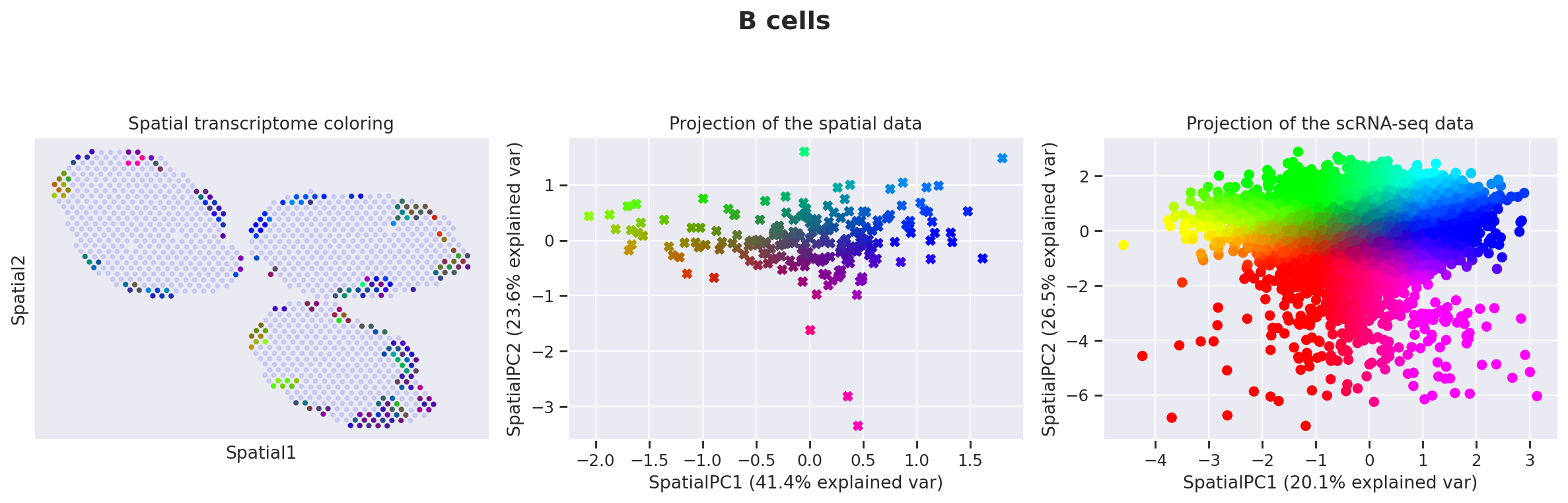
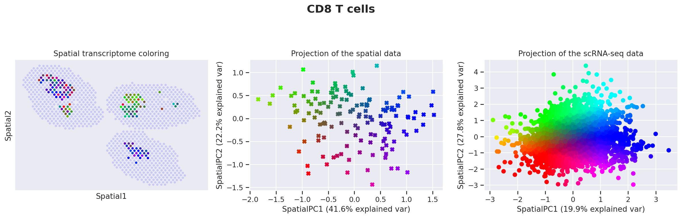
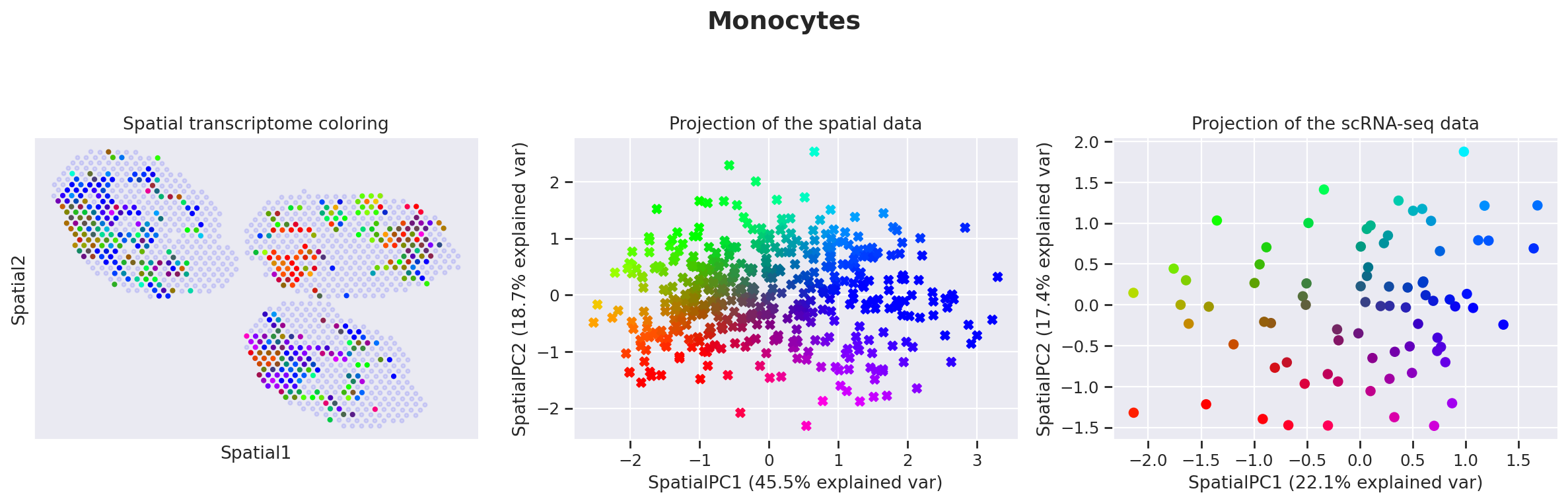
Because those values may be hard to examine manually for end-users, we presented in the manuscript several methods for prioritizing the study of different cell types (based on spatially-weighted PCA and Hotspot). Below we provide the result of our automated pipeline with the spatially-weighted PCA.

More precisely, for de novo detection of spatial patterns, we study the gamma space and use a spatially-informed PCA to find the spatial axis of variation in this gamma space. We use EnrichR to functionally annotate these genes. In particular, we recover enrichment of IFN genes across monocytes as well as B cells

The function explore_gamma_space operates as follow, for each cell type individually:

1. Select all the spots with proportions beyond the magnitude threshold,

2. Calculate the spot-specific cell-type-specific embeddings gamma,

3. Calculate the first two principal vectors of those gamma values, weighted by the spatial coordinates,

4. Project all the embeddings (considered spots, and single-cell profiles) onto this 2D space,

5. Map each spot (or cell) to a specific color via its 2d coordinate, using the cmap2d package

6. Plot (A) the color of every spot in spatial coordinates (B) the color of every spot in sPC space (C) the color of every single cell in sPC space

7. Calculate genes enriched in each direction and group into pathways with EnrichR

destvi_utils.explore_gamma_space(st_model, sc_model, ct_list=ct_list, ct_thresholds=ct_thresholds)

Genes associated with SpatialPC1

Positively

---------------------------------------------------------------------------------------

Cd74, H2-Aa, H2-Eb1, Cd79a, H2-Ab1, Fth1, Mef2c, Fcer2a, Fcmr, Iglc2, Igkc, Ighm, Rpsa, Ly6d, Tmsb4x, Vpreb3, 
Iglc3, Junb, Ftl1, Rplp1, Fcrla, Apoe, Chchd10, Ctsh, S100a10, Srgn, Fos, Ms4a1, Napsa, Pxdc1, H2-DMb1, Cd81, 
Gm26532, Lsp1, Plekho1, Serpinb1a, Mzb1, Rpl41, Gm42418, Cd200, Crip1, Cst3, Hexb, Fcgrt, Plk2, Gsn, Gpr183, Ciita,
Dusp1, Sfn

---------------------------------------------------------------------------------------

Antigen-activated B-cell receptor generation of second messengers*, BDNF signaling pathway*, Immune system*, 
Immunoregulatory interactions between a lymphoid and a non-lymphoid cell*, Adaptive immune system*, Signaling by 
the B cell receptor (BCR)*, TSH regulation of gene expression*, T cell receptor regulation of apoptosis*, ERBB1 
downstream pathway*, Wnt interactions in lipid metabolism and immune response*

Negatively

---------------------------------------------------------------------------------------

Stat1, Ifit3, Zbp1, Ifi47, Rtp4, Isg15, Irf7, Trim30a, Usp18, Slfn5, Ifit3b, Bst2, Ifit1, Igtp, Phf11b, Mki67, 
Gbp7, Birc5, Ifit2, Ccna2, Kif11, Parp14, Rnf213, Tpx2, Nusap1, Oas3, Rrm2, Hmmr, Rsad2, Eif2ak2, Gbp4, Esco2, 
Ncapg, Isg20, Ube2c, Oasl2, Kif4, Cdca3, Lgals3bp, Cdk1, Hist1h3c, Cdca5, Ccnb2, Cenpf, Serpina3g, E2f8, Rad51ap1, 
Plk1, Kif22, Bub1

---------------------------------------------------------------------------------------

Interferon signaling*, Interferon alpha/beta signaling*, Immune system signaling by interferons, interleukins, 
prolactin, and growth hormones*, Immune system*, FOXM1 transcription factor network*, Cyclin A/B1-associated events
during G2/M transition*, Antiviral mechanism by interferon-stimulated genes*, Cell cycle*, Progesterone-mediated 
oocyte maturation*, Interferon-gamma signaling pathway*

Genes associated with SpatialPC2

Positively

---------------------------------------------------------------------------------------

Cd79a, H2-Eb1, Cd74, H2-Aa, H2-Ab1, Ighm, Ly6d, Malat1, Ms4a1, Mef2c, Fth1, Iglc3, Igkc, Iglc2, Fcer2a, Fcmr, 
Rnase6, Fcrla, Ctsh, Mzb1, Vpreb3, Itm2b, Gm42418, Napsa, Ifit3, Slfn5, Ly86, Serpinb1a, Bcl11a, Srgn, Cd38, Jun, 
Irf7, Cst3, Ifi27l2a, Tspo, Crip1, Hspa1b, Pkib, Ly6a, Lsp1, Oasl2, Fcgrt, Icosl, Unc93b1, B2m, Ciita, Rtp4, Hexb, 
Hist1h1c

---------------------------------------------------------------------------------------

Immune system*, Antigen-activated B-cell receptor generation of second messengers*, Innate immune system*, 
Signaling by the B cell receptor (BCR)*, Toll receptor cascades*, Antigen processing and presentation*, Adaptive 
immune system*, Immunoregulatory interactions between a lymphoid and a non-lymphoid cell*, Amyloids*, Interferon 
signaling

Negatively

---------------------------------------------------------------------------------------

Birc5, Ccna2, Ube2c, Tpx2, Rrm2, Cdk1, Ccnb2, Mki67, Cdca3, Kif11, Hmmr, Ncapg, Bub1, Plk1, Cks1b, Uhrf1, Cdca8, 
Kif4, Ncaph, Ccnb1, Cdkn3, Kif2c, Hist1h3c, Ppp1r14b, Pbk, Spc24, Ska1, Kif22, Tyms, Neil3, Melk, Esco2, Dctpp1, 
Prc1, Cenpf, Cdca5, Top2a, Srm, Bzw2, Nuf2, Kif20a, E2f8, Cdca2, Cep55, Kif15, Mxd3, Lcp2, Nusap1, Nme1, Stmn1

---------------------------------------------------------------------------------------

Cell cycle*, M phase pathway*, Aurora B signaling*, FOXM1 transcription factor network*, Polo-like kinase 1 (PLK1) 
pathway*, DNA replication*, Cyclin A/B1-associated events during G2/M transition*, Kinesins*, Mitotic G1-G1/S 
phases*, Mitotic prometaphase*

Genes associated with SpatialPC1

Positively

---------------------------------------------------------------------------------------

Ccl5, Ly6c2, Ifit3, Ctla2a, Xcl1, S100a6, Klrc2, Samd3, Cxcr3, Ms4a4c, Il18rap, Oasl2, Ccr5, Klrk1, Klre1, Klrc1, 
Ifit1, Irf7, 1700025G04Rik, Isg15, Rsad2, Slamf7, Dennd4a, Eomes, Serpina3g, Rtp4, Trim30a, Fcer1g, Gbp7, Ifngr1, 
Gbp4, Lrrk1, Il18r1, Ly6a, Il2rb, Usp18, Ifit3b, Zbp1, Plek, Igtp, AW112010, Parp14, Cd44, Gbp2, Sidt1, Herc6, 
Ctla2b, Gzmm, Klra7, Oas3

---------------------------------------------------------------------------------------

Interferon signaling*, Immune system signaling by interferons, interleukins, prolactin, and growth hormones*, 
Interferon alpha/beta signaling*, Interferon-gamma signaling pathway*, Immune system*, Interleukin-2 signaling 
pathway*, Cytokine-cytokine receptor interaction*, Selective expression of chemokine receptors during T-cell 
polarization*, Interleukin-12-mediated signaling events*, Interleukin-12/STAT4 pathway*

Negatively

---------------------------------------------------------------------------------------

Cd8b1, Ppia, Rgcc, Rplp0, Cd3g, Cd8a, Npc2, Ramp1, Rpl41, Rps2, Ccr9, Igfbp4, Rpsa, Lef1, Trac, Itgae, Rplp1, Cd3d,
Lat, Actn2, Actg1, Trbc2, Cd3e, Ptma, Actb, Nme2, Tubb5, Actn1, Eif4a1, Npm1, Inpp4b, Timp2, Tmsb4x, Dapl1, Ddit4, 
Thy1, Slc25a5, Dtx1, Plekho1, Ybx1, Rgs10, Cd226, Ftl1, Calm1, Sh3bp1, Ran, Lsp1, Gpr68, Cyb5a, Hnrnpa1

---------------------------------------------------------------------------------------

T helper cell surface molecules*, MEF2D role in T cell apoptosis*, Generation of second messenger molecules*, 
Interleukin-17 signaling pathway*, Disease*, T cell receptor signaling in naive CD8+ T cells*, Immunoregulatory 
interactions between a lymphoid and a non-lymphoid cell*, PD-1 signaling*, Adherens junction cell adhesion*, 
Arrhythmogenic right ventricular cardiomyopathy (ARVC)*

Genes associated with SpatialPC2

Positively

---------------------------------------------------------------------------------------

Ccl5, Ly6c2, Rpsa, Cxcr3, Ctla2a, Rps12, Samd3, Hopx, Xcl1, Gzmm, 1700025G04Rik, Rplp0, Il2rb, Rps2, Rplp1, Cd44, 
Ahnak, Ifitm10, Plek, Ifngr1, Sidt1, Il18rap, Ccr5, Klrd1, Ctla2b, Pglyrp1, Gpr183, S100a6, Il18r1, Il7r, Eomes, 
H2afz, Bbc3, Lrrk1, Rpl41, Klra7, Zyx, Runx2, Dennd4a, Klre1, Itgb1, Myo1f, Ccr2, Bcl2, Itm2a, Slamf7, Klrc2, Ccl4,
Ms4a4c, Klrc1

---------------------------------------------------------------------------------------

Interleukin-2 signaling pathway*, Cytokine-cytokine receptor interaction*, T cell receptor regulation of 
apoptosis*, Binding of chemokines to chemokine receptors*, Selective expression of chemokine receptors during 
T-cell polarization*, Cytoplasmic ribosomal proteins*, Leptin influence on immune response*, Ras-independent 
pathway in NK cell-mediated cytotoxicity*, Interleukin-12-mediated signaling events*, Influenza viral RNA 
transcription and replication*

Negatively

---------------------------------------------------------------------------------------

Isg15, Ifit1, Ccr9, Stat1, Zbp1, Ifit3, Iigp1, Slfn5, Ifi27l2a, Igtp, Isg20, Ramp1, Rgcc, Rtp4, Gbp2, Rsad2, 
Ifit3b, Gbp7, Oasl2, Usp18, Itgae, Gbp4, Malat1, Irf7, B2m, Gbp8, Parp14, Ifi47, Slfn1, Bst2, Rnf213, Ddx60, Cmpk2,
Oas3, Ly6a, Trim30a, Herc6, Cd3g, Igfbp4, Ifih1, Pmepa1, Cd274, Sox4, Trafd1, Eif2ak2, Actb, Lgals3bp, Phf11b, 
Art2b, Cd226

---------------------------------------------------------------------------------------

Interferon signaling*, Interferon alpha/beta signaling*, Immune system signaling by interferons, interleukins, 
prolactin, and growth hormones*, Immune system*, Interferon-gamma signaling pathway*, Antiviral mechanism by 
interferon-stimulated genes*, Type II interferon signaling (interferon-gamma)*, CTL mediated immune response 
against target cells, TRAF3-dependent IRF activation pathway, Interleukin-12-mediated signaling events

Genes associated with SpatialPC1

Positively

---------------------------------------------------------------------------------------

Tspan3, Sema7a, Cd63, Plxnc1, Fabp5, Dbf4, Ftsj3, Itgax, Mif, Nr4a3, Abcd2, Ehd1, Tarm1, Fcrl5, Vegfa, Hnrnpll, 
Hdgf, Plxna1, Fosb, Fosl2, Tuba1c, Ccdc88a, Itga8, Il1b, St3gal5, Rgs1, Fen1, Nrp2, Canx, Eprs, Rpl41, Hnrnpab, 
Sirpa, Rad21, Psrc1, Klra17, Klrb1b, Tuba1a, Bcl2l1, Dusp1, Ank, Cyfip1, Basp1, Gla, Ppia, Osm, Neat1, Gria3, 
Actn1, Inpp4b

---------------------------------------------------------------------------------------

Interleukin-2 signaling pathway*, Other semaphorin interactions*, EGFR1 pathway*, Response to elevated platelet 
cytosolic calcium*, Neurophilin interactions with VEGF and VEGF receptor*, Hemostasis pathway*, Signaling by VEGF, 
HIV life cycle early phase, Semaphorin interactions, AP-1 transcription factor network

Negatively

---------------------------------------------------------------------------------------

Ifi204, Ms4a6b, Ifit3, Plac8, Igtp, Ifi205, Fcgr1, Oasl2, Igkc, Ms4a4c, Sp140, Ifit3b, Ifi47, Flt1, Rtp4, Oas3, 
Zbp1, Gbp2, Nupr1, Scimp, Gnb4, Themis2, Ms4a1, Ms4a6d, Ifit1, Gbp7, Ccr2, Hivep3, Psme2, Irf1, Cxcl10, Rnf213, 
Iglc2, Cybb, Ctss, Arhgap31, Trafd1, Ly6d, Ly6c2, Ms4a6c, Ms4a4b, Slfn1, Bst2, Pou2af1, Ifit2, Lyz2, Cd24a, Isg20, 
Unc93b1, Vpreb3

---------------------------------------------------------------------------------------

Interferon alpha/beta signaling*, Immune system*, Interferon signaling*, Immune system signaling by interferons, 
interleukins, prolactin, and growth hormones*, Type II interferon signaling (interferon-gamma)*, Innate immune 
system*, Thymic stromal lymphopoietin (TSLP) pathway*, Interferon-gamma signaling pathway*, Toll-like receptor 
endosomal trafficking and processing*, Antigen processing: cross presentation

Genes associated with SpatialPC2

Positively

---------------------------------------------------------------------------------------

Glrx, Anpep, Klrk1, Fgl2, Ranbp1, Clic4, Cxcl9, Csrp1, Hells, Pnp, Isg15, Calm1, Cfb, Naaa, Mxd1, Cks1b, Pdk3, 
Mcm10, Spint1, Rps27l, Chaf1a, H2-DMb1, Il1rn, Hspa9, Evi2a, Cycs, Alyref, Cd40, Apex1, Efhd2, Psma4, Ccnd1, Sub1, 
Cdkn1a, Parp12, Slamf8, Tmpo, Ctsc, Gatm, Atpif1, Rfc4, Mvp, Slco3a1, Gapdh, Plekho2, Anxa4, E2f1, Mcm4, Ywhae, 
Lgals1

---------------------------------------------------------------------------------------

Mitotic G1-G1/S phases*, S phase*, Cell cycle*, T cell receptor regulation of apoptosis*, EGFR1 pathway*, Cyclin 
D-associated events in G1*, DNA replication pre-Initiation*, Cell cycle checkpoints*, DNA replication*, Glioma*

Negatively

---------------------------------------------------------------------------------------

Fcmr, Fcrla, Itgb5, Cx3cr1, Hfe, Pou2af1, Iglc3, Ms4a1, Mzb1, Igkc, Ifngr1, Iglc2, Blk, Cd79a, Gfra2, Ctsb, Csf1r, 
Ly75, Spn, Prkar1b, Itm2b, Myc, Ighm, Ly6d, Egr3, Ace, Vpreb3, Gm1673, Cd200, Tmem26, Mef2c, Zbtb20, Nrgn, Chek1, 
Ifng, Il1r1, 3830403N18Rik, Fcer2a, Msrb1, Myb, Mgst1, Tlr13, Slc8b1, Cacna1b, Klk8, Serpinb1a, Art2b, Cdkn2c, 
Hjurp, Gm5547

---------------------------------------------------------------------------------------

Antigen-activated B-cell receptor generation of second messengers*, Immune system*, Signaling by the B cell 
receptor (BCR)*, Adaptive immune system*, Inhibition of activated T cell apoptosis by neuropeptides VIP and PACAP*,
TSH regulation of gene expression*, T cell receptor regulation of apoptosis*, Interleukin-2 signaling pathway*, 
Immunoregulatory interactions between a lymphoid and a non-lymphoid cell*, Cytokine-cytokine receptor interaction

We anticipate this to be a valuable ressource for formulating scientific hypotheses from ST data.

Example with B cells; and differential expression

First, we display the genes identified via the pipeline as well as Hotspot (see manuscript), using the B-cell-specific gene expression values imputed by DestVI.

plt.figure(figsize=(8, 8))

ct_name = "B cells"
gene_name = ["Ifit3", "Ifit3b", "Ifit1", "Isg15", "Oas3", "Usp18", "Isg20"]

# we must filter spots with low abundance (consult the paper for an automatic procedure)
indices = np.where(st_adata.obsm["proportions"][ct_name].values > 0.2)[0]

# impute genes and combine them
specific_expression = np.sum(st_model.get_scale_for_ct(ct_name, indices=indices)[gene_name], 1)
specific_expression = np.log(1 + 1e4 * specific_expression)

# plot (i) background (ii) g
plt.scatter(st_adata.obsm["location"][:, 0], st_adata.obsm["location"][:, 1], alpha=0.05)
plt.scatter(
    st_adata.obsm["location"][indices][:, 0],
    st_adata.obsm["location"][indices][:, 1],
    c=specific_expression,
    s=10,
    cmap="Reds",
)
plt.colorbar()
plt.title(f"Imputation of {gene_name} in {ct_name}")
plt.show()

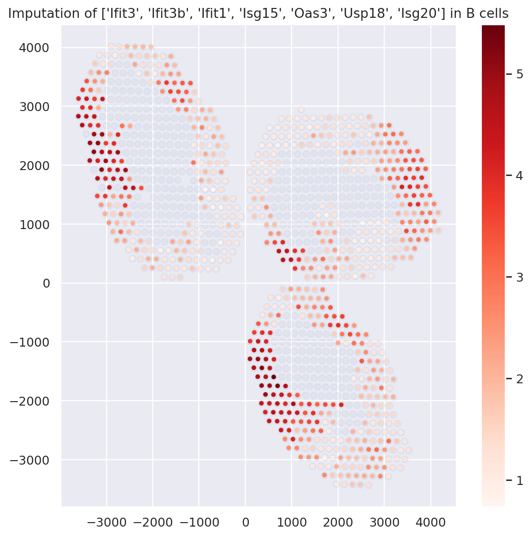
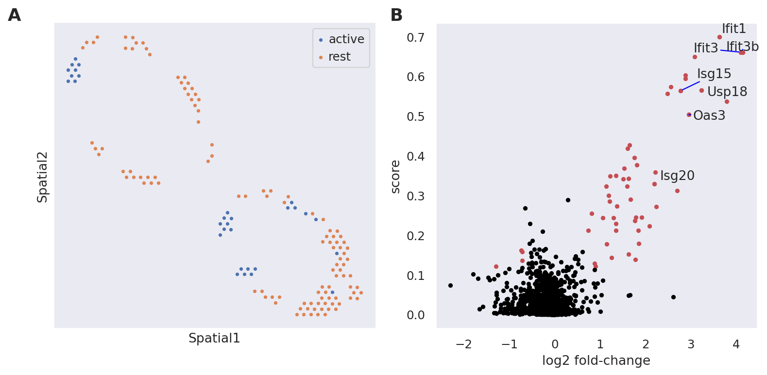
Second, we apply a Kolmogorov-Smirnov test on the generated counts to study the differential expression of B cells in the exposed lymph nodes, between the interfollicular area (IFA) and the rest. We display the identified IFN genes in a Volcano plot and see significant upregulation in the IFA area of exposed lymph nodes.

ct = "B cells"
imputation = st_model.get_scale_for_ct(ct)
color = np.log(1 + 1e5 * imputation["Ifit3"].values)
threshold = 4

mask = np.logical_and(
    np.logical_or(st_adata.obs["LN"] == "TC", st_adata.obs["LN"] == "BD"),
    color > threshold,
).values

mask2 = np.logical_and(
    np.logical_or(st_adata.obs["LN"] == "TC", st_adata.obs["LN"] == "BD"),
    color < threshold,
).values

_ = destvi_utils.de_genes(
    st_model, mask=mask, mask2=mask2, threshold=ct_thresholds[ct], ct=ct, key="IFN_rich"
)

display(st_adata.uns["IFN_rich"]["de_results"].head(10))

destvi_utils.plot_de_genes(
    st_adata,
    interesting_genes=["Ifit3", "Ifit3b", "Ifit1", "Isg15", "Oas3", "Usp18", "Isg20"],
    key="IFN_rich",
)

	log2FC	score	pval
Ifit1	4.032940	0.729527	0.0
Ifit3	4.342963	0.715804	0.0
Ifit2	3.490396	0.664848	0.0
Ifit3b	4.326105	0.602065	0.0
Slfn5	3.020566	0.593361	0.0
Ifitm3	3.304686	0.591831	0.0
Irf7	2.533088	0.550693	0.0
Oas3	3.037543	0.545928	0.0
Cmpk2	2.569157	0.542041	0.0
Isg15	3.052167	0.514476	0.0