Use pretrained models of scVI-hub for Tahoe100M

This notebook represent an example of how to perform downstream anaylsis on a pretrained SCVI model that was minified and saved in a model hub. In this case we use the model that was trained based on the Tahoe100M dataset , by Vevo Therapuetics. See link to model hub here

Steps performed:

1. Loading the minified data from AWS

2. Setting up minified model with minified data

3. Visualize the latent space

4. Perform differential expression and visualize with interactive volcano plot and heatmap using Plotly

import tempfile

import matplotlib.pyplot as plt
import numpy as np
import pandas as pd
import scanpy as sc
import scvi
import scvi.hub
import seaborn as sns
import torch

scvi.settings.seed = 0
print("Last run with scvi-tools version:", scvi.__version__)

Last run with scvi-tools version: 1.3.2

sc.set_figure_params(figsize=(6, 6), frameon=False)
sns.set_theme()
torch.set_float32_matmul_precision("high")
save_dir = tempfile.TemporaryDirectory()

%config InlineBackend.print_figure_kwargs={"facecolor": "w"}
%config InlineBackend.figure_format="retina"

Get the data

We start by downloading the model from its hub. Note that the model is very large therefore it will take time to being download.

tahoe_hubmodel = scvi.hub.HubModel.pull_from_huggingface_hub(
    repo_name="vevotx/Tahoe-100M-SCVI-v1", cache_dir="."
)

We can see the model card

# This will be a bit long to scroll, but has all the info
# tahoe_hubmodel

We will extract he model and the minifed adata

tahoe = tahoe_hubmodel.model
tahoe

INFO     Loading model...                                                                                          
INFO     File ./models--vevotx--Tahoe-100M-SCVI-v1/snapshots/b5283a73fbbed812a95264ace360da538b20af89/model.pt     
         already downloaded

SCVI model with the following parameters: 
n_hidden: 128, n_latent: 10, n_layers: 1, dropout_rate: 0.1, dispersion: gene, gene_likelihood: nb, 
latent_distribution: normal.
Training status: Trained
Model's adata is minified?: True

tahoe.adata

AnnData object with n_obs × n_vars = 95624334 × 62710
    obs: 'sample', 'species', 'gene_count', 'tscp_count', 'mread_count', 'bc1_wind', 'bc2_wind', 'bc3_wind', 'bc1_well', 'bc2_well', 'bc3_well', 'id', 'drugname_drugconc', 'drug', 'INT_ID', 'NUM.SNPS', 'NUM.READS', 'demuxlet_call', 'BEST.LLK', 'NEXT.LLK', 'DIFF.LLK.BEST.NEXT', 'BEST.POSTERIOR', 'SNG.POSTERIOR', 'SNG.BEST.LLK', 'SNG.NEXT.LLK', 'SNG.ONLY.POSTERIOR', 'DBL.BEST.LLK', 'DIFF.LLK.SNG.DBL', 'sublibrary', 'BARCODE', 'pcnt_mito', 'S_score', 'G2M_score', 'phase', 'pass_filter', 'dataset', '_scvi_batch', '_scvi_labels', '_scvi_observed_lib_size', 'plate', 'Cell_Name_Vevo', 'Cell_ID_Cellosaur', 'observed_lib_size'
    var: 'gene_id', 'genome', 'SUB_LIB_ID'
    uns: '_scvi_adata_minify_type', '_scvi_manager_uuid', '_scvi_uuid'
    obsm: 'X_latent_qzm', 'X_latent_qzv', 'scvi_latent_qzm', 'scvi_latent_qzv'
    layers: 'counts'

tahoe.view_anndata_setup()

Anndata setup with scvi-tools version 1.3.2.

Setup via `SCVI.setup_anndata` with arguments:

{
│   'layer': 'counts',
│   'batch_key': None,
│   'labels_key': None,
│   'size_factor_key': 'tscp_count',
│   'categorical_covariate_keys': None,
│   'continuous_covariate_keys': None
}

          Summary Statistics           
┏━━━━━━━━━━━━━━━━━━━━━━━━━━┳━━━━━━━━━━┓
┃     Summary Stat Key     ┃  Value   ┃
┡━━━━━━━━━━━━━━━━━━━━━━━━━━╇━━━━━━━━━━┩
│         n_batch          │    1     │
│         n_cells          │ 95624334 │
│ n_extra_categorical_covs │    0     │
│ n_extra_continuous_covs  │    0     │
│         n_labels         │    1     │
│       n_latent_qzm       │    10    │
│       n_latent_qzv       │    10    │
│          n_vars          │  62710   │
└──────────────────────────┴──────────┘

                       Data Registry                        
┏━━━━━━━━━━━━━━━━━━━┳━━━━━━━━━━━━━━━━━━━━━━━━━━━━━━━━━━━━━━┓
┃   Registry Key    ┃         scvi-tools Location          ┃
┡━━━━━━━━━━━━━━━━━━━╇━━━━━━━━━━━━━━━━━━━━━━━━━━━━━━━━━━━━━━┩
│         X         │        adata.layers['counts']        │
│       batch       │       adata.obs['_scvi_batch']       │
│      labels       │      adata.obs['_scvi_labels']       │
│    latent_qzm     │    adata.obsm['scvi_latent_qzm']     │
│    latent_qzv     │    adata.obsm['scvi_latent_qzv']     │
│    minify_type    │ adata.uns['_scvi_adata_minify_type'] │
│ observed_lib_size │    adata.obs['observed_lib_size']    │
│    size_factor    │       adata.obs['tscp_count']        │
└───────────────────┴──────────────────────────────────────┘

                     batch State Registry                      
┏━━━━━━━━━━━━━━━━━━━━━━━━━━┳━━━━━━━━━━━━┳━━━━━━━━━━━━━━━━━━━━━┓
┃     Source Location      ┃ Categories ┃ scvi-tools Encoding ┃
┡━━━━━━━━━━━━━━━━━━━━━━━━━━╇━━━━━━━━━━━━╇━━━━━━━━━━━━━━━━━━━━━┩
│ adata.obs['_scvi_batch'] │     0      │          0          │
└──────────────────────────┴────────────┴─────────────────────┘

                     labels State Registry                      
┏━━━━━━━━━━━━━━━━━━━━━━━━━━━┳━━━━━━━━━━━━┳━━━━━━━━━━━━━━━━━━━━━┓
┃      Source Location      ┃ Categories ┃ scvi-tools Encoding ┃
┡━━━━━━━━━━━━━━━━━━━━━━━━━━━╇━━━━━━━━━━━━╇━━━━━━━━━━━━━━━━━━━━━┩
│ adata.obs['_scvi_labels'] │     0      │          0          │
└───────────────────────────┴────────────┴─────────────────────┘

# from pprint import pprint
# pprint(tahoe.registry)

Get the latent space

SCVI_LATENT_KEY = "X_scVI"
latent = tahoe.get_latent_representation()
tahoe.adata.obsm[SCVI_LATENT_KEY] = latent
latent.shape

(95624334, 10)

# we visualize a subset of the results to avoid meaningless overplotting.
subset_adata = tahoe.adata[np.random.randint(0, tahoe.adata.shape[0], (1_000_000,))]
subset_adata

View of AnnData object with n_obs × n_vars = 1000000 × 62710
    obs: 'sample', 'species', 'gene_count', 'tscp_count', 'mread_count', 'bc1_wind', 'bc2_wind', 'bc3_wind', 'bc1_well', 'bc2_well', 'bc3_well', 'id', 'drugname_drugconc', 'drug', 'INT_ID', 'NUM.SNPS', 'NUM.READS', 'demuxlet_call', 'BEST.LLK', 'NEXT.LLK', 'DIFF.LLK.BEST.NEXT', 'BEST.POSTERIOR', 'SNG.POSTERIOR', 'SNG.BEST.LLK', 'SNG.NEXT.LLK', 'SNG.ONLY.POSTERIOR', 'DBL.BEST.LLK', 'DIFF.LLK.SNG.DBL', 'sublibrary', 'BARCODE', 'pcnt_mito', 'S_score', 'G2M_score', 'phase', 'pass_filter', 'dataset', '_scvi_batch', '_scvi_labels', '_scvi_observed_lib_size', 'plate', 'Cell_Name_Vevo', 'Cell_ID_Cellosaur', 'observed_lib_size'
    var: 'gene_id', 'genome', 'SUB_LIB_ID'
    uns: '_scvi_adata_minify_type', '_scvi_manager_uuid', '_scvi_uuid'
    obsm: 'X_latent_qzm', 'X_latent_qzv', 'scvi_latent_qzm', 'scvi_latent_qzv', 'X_scVI'
    layers: 'counts'

subset_adata.X.shape

(1000000, 62710)

import gc

gc.collect()

0

Exploritory Analysis

tahoe.adata.obs.head()

	sample	species	gene_count	tscp_count	mread_count	bc1_wind	bc2_wind	bc3_wind	bc1_well	bc2_well	...	phase	pass_filter	dataset	_scvi_batch	_scvi_labels	_scvi_observed_lib_size	plate	Cell_Name_Vevo	Cell_ID_Cellosaur	observed_lib_size
BARCODE_SUB_LIB_ID
01_001_052-lib_1105	smp_1783	hg38	1878	2893	3284	1	1	52	A1	A1	...	G2M	full	0	0	0	2893	4	PANC-1	CVCL_0480	2893
01_001_105-lib_1105	smp_1783	hg38	1765	2434	2764	1	1	105	A1	A1	...	G2M	full	0	0	0	2434	4	SW480	CVCL_0546	2434
01_001_165-lib_1105	smp_1783	hg38	3174	5691	6454	1	1	165	A1	A1	...	G2M	full	0	0	0	5691	4	SW1417	CVCL_1717	5691
01_003_094-lib_1105	smp_1783	hg38	1380	1804	2050	1	3	94	A1	A3	...	G2M	full	0	0	0	1804	4	SW1417	CVCL_1717	1804
01_003_164-lib_1105	smp_1783	hg38	1179	1514	1715	1	3	164	A1	A3	...	G1	full	0	0	0	1514	4	A498	CVCL_1056	1514

5 rows × 43 columns

# confuison table of plates and cell type (they are spread evently)
pd.crosstab(subset_adata.obs.plate, subset_adata.obs.Cell_ID_Cellosaur)

Cell_ID_Cellosaur	CVCL_0023	CVCL_0332	CVCL_0292	CVCL_1285	CVCL_0069	CVCL_1056	CVCL_1381	CVCL_0218	CVCL_0320	CVCL_0546	...	CVCL_0371	CVCL_0099	CVCL_0028	CVCL_1550	CVCL_0131	CVCL_C466	CVCL_1547	CVCL_1495	CVCL_1531	CVCL_1517
plate
1	1605	866	785	1649	699	1172	1128	1056	1648	3410	...	1543	473	285	1427	1423	1406	1049	905	23	1771
2	2331	1249	1288	2660	1063	1856	1624	1344	2035	5109	...	2093	679	494	1970	2240	1911	1606	1311	25	2282
3	1286	817	475	1533	538	1123	1031	537	1131	2394	...	1341	326	241	1520	1559	785	903	716	21	1570
4	2181	1157	1044	2310	1093	1867	1616	1089	1681	4242	...	1741	645	530	1734	2014	1361	1612	1274	30	1752
5	1931	1209	684	2282	1056	1975	1560	786	1463	3108	...	1361	532	546	1690	2210	1157	1417	1194	36	1727
6	2321	1122	1261	2508	1307	1935	1811	1153	1689	4736	...	1774	814	759	1763	2212	1754	1541	1364	26	1748
7	1379	1147	796	2001	968	1843	1492	693	1149	3210	...	1176	800	246	1408	1015	755	942	1200	10	764
8	2063	1550	1696	2856	1642	2380	2062	1472	1898	6383	...	2122	1664	443	1886	1592	1171	1460	1885	20	1018
9	1340	1084	1019	1896	967	1702	1322	924	1348	4024	...	1415	862	294	1291	1112	793	900	1212	13	846
10	1945	1537	1342	2968	1433	2434	1897	1241	1732	5459	...	1712	1232	396	1647	1474	1201	1340	1657	19	1143
11	1843	1716	1122	2866	1097	2602	1616	1083	1671	4643	...	1593	991	248	1462	1464	1302	1281	1596	14	1188
12	2616	1963	1863	3943	1876	3353	2500	1444	2108	7034	...	2194	1846	621	2051	1981	1644	1710	2084	16	1296
13	2026	1555	1568	2931	1638	2619	2005	1245	1728	5560	...	1844	1444	410	1937	1610	1156	1324	1784	21	1024
14	1814	1028	887	2220	939	1808	1274	1170	1604	3967	...	1618	528	371	1331	2011	1339	1338	1124	23	1901

14 rows × 50 columns

# integration of drugs and cell type (certain type of cancer are given certian type of drugs)
df = subset_adata.obs.groupby(["drug", "Cell_ID_Cellosaur"]).size().unstack(fill_value=0)
norm_df = df / df.sum(axis=0)
plt.figure(figsize=(8, 8))
_ = plt.pcolor(norm_df)
_ = plt.xticks(np.arange(0.5, len(df.columns), 1), df.columns, rotation=90)
_ = plt.yticks(np.arange(0.5, len(df.index), 1), df.index)
plt.xlabel("Cell_ID_Cellosaur")
plt.ylabel("drug")

Text(0, 0.5, 'drug')

Visualization with batch correction (scVI)

gc.collect()

0

# use scVI latent space for UMAP generation
sc.pp.neighbors(subset_adata, use_rep=SCVI_LATENT_KEY)
sc.tl.umap(subset_adata, min_dist=0.3)

# because we have so many drugs, we wont plot the umap here
# sc.pl.umap(
#    subset_adata,
#    color=["drug"],
#    frameon=False,
# )

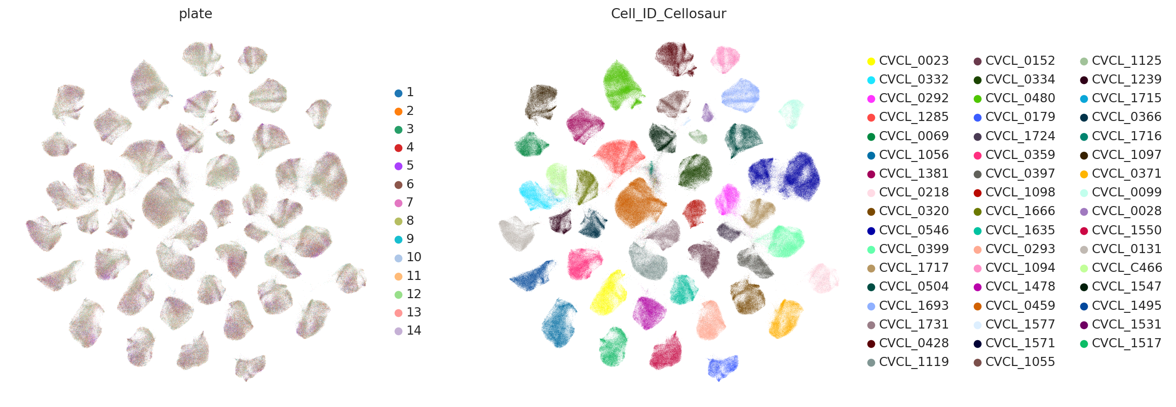
sc.pl.umap(
    subset_adata,
    color=["plate", "Cell_ID_Cellosaur"],
    ncols=2,
    frameon=False,
)

Visualization PCA

In order to save time we will subset the data even further

subset_adata2 = subset_adata[np.random.randint(0, subset_adata.shape[0], (100_000,))]
subset_adata2

View of AnnData object with n_obs × n_vars = 100000 × 62710
    obs: 'sample', 'species', 'gene_count', 'tscp_count', 'mread_count', 'bc1_wind', 'bc2_wind', 'bc3_wind', 'bc1_well', 'bc2_well', 'bc3_well', 'id', 'drugname_drugconc', 'drug', 'INT_ID', 'NUM.SNPS', 'NUM.READS', 'demuxlet_call', 'BEST.LLK', 'NEXT.LLK', 'DIFF.LLK.BEST.NEXT', 'BEST.POSTERIOR', 'SNG.POSTERIOR', 'SNG.BEST.LLK', 'SNG.NEXT.LLK', 'SNG.ONLY.POSTERIOR', 'DBL.BEST.LLK', 'DIFF.LLK.SNG.DBL', 'sublibrary', 'BARCODE', 'pcnt_mito', 'S_score', 'G2M_score', 'phase', 'pass_filter', 'dataset', '_scvi_batch', '_scvi_labels', '_scvi_observed_lib_size', 'plate', 'Cell_Name_Vevo', 'Cell_ID_Cellosaur', 'observed_lib_size'
    var: 'gene_id', 'genome', 'SUB_LIB_ID'
    uns: '_scvi_adata_minify_type', '_scvi_manager_uuid', '_scvi_uuid', 'neighbors', 'umap', 'plate_colors', 'Cell_ID_Cellosaur_colors'
    obsm: 'X_latent_qzm', 'X_latent_qzv', 'scvi_latent_qzm', 'scvi_latent_qzv', 'X_scVI', 'X_umap'
    layers: 'counts'
    obsp: 'distances', 'connectivities'

# run PCA then generate UMAP plots (here no results will be shown as no raw data exists)
sc.tl.pca(subset_adata2)
sc.pp.neighbors(subset_adata2, n_pcs=50, n_neighbors=50)
sc.tl.umap(subset_adata2, min_dist=0.1)

# sc.pl.umap(
#    subset_adata2,
#    color=["plate", "Cell_ID_Cellosaur"],
#    frameon=False,
# )

Clustering on the scVI latent space

# neighbors were already computed using scVI
SCVI_CLUSTERS_KEY = "leiden_scVI"
sc.tl.leiden(subset_adata, key_added=SCVI_CLUSTERS_KEY, resolution=0.5)

sc.pl.umap(
    subset_adata,
    color=[SCVI_CLUSTERS_KEY],
    frameon=False,
)

# integration of leiden clsuters and cell type
df = subset_adata.obs.groupby(["leiden_scVI", "Cell_ID_Cellosaur"]).size().unstack(fill_value=0)
norm_df = df / df.sum(axis=0)
plt.figure(figsize=(8, 8))
_ = plt.pcolor(norm_df)
_ = plt.xticks(np.arange(0.5, len(df.columns), 1), df.columns, rotation=90)
_ = plt.yticks(np.arange(0.5, len(df.index), 1), df.index)
plt.xlabel("Cell_ID_Cellosaur")
plt.ylabel("leiden_scVI")

Text(0, 0.5, 'leiden_scVI')

SCANVI

Running scanvi from the scvi model will require the original counts matrix and cant be done, as count matrix is all 0.

gc.collect()

0

tahoe.save("tahoe_tmp", save_anndata=True, overwrite=True)

tahoe_loaded = scvi.model.SCVI.load("tahoe_tmp", adata=tahoe.adata)

INFO     File tahoe_tmp/model.pt already downloaded

tahoe_loaded.minify_adata(minified_data_type="latent_posterior_parameters_with_counts")

INFO     Input AnnData not setup with scvi-tools. attempting to transfer AnnData setup                             
INFO     Generating sequential column names                                                                        
INFO     Generating sequential column names

# predict on drug?
tahoe_scanvi = scvi.model.SCANVI.from_scvi_model(
    tahoe_loaded,
    unlabeled_category="Unknown",
    labels_key="drug",
)

tahoe_loaded.adata.X

<Compressed Sparse Row sparse matrix of dtype 'float64'
	with 0 stored elements and shape (95624334, 62710)>

# tahoe_scanvi.train(max_epochs=5,batch_size=64) #this fails in the workstation

predictions = tahoe_scanvi.predict(subset_adata)
subset_adata.obs["predictions_scanvi"] = predictions
# predictions

INFO     Input AnnData not setup with scvi-tools. attempting to transfer AnnData setup

See the predictions confusion matrix

df = subset_adata.obs.groupby(["drug", "predictions_scanvi"]).size().unstack(fill_value=0)
norm_df = df / df.sum(axis=0)

print("The overall Accuracy is:", np.round(np.trace(norm_df), 2))

The overall Accuracy is: 0.63

We create the scanvi embeddings as well (if model was trained)

SCANVI_LATENT_KEY = "X_scanVI"
# latent_scanvi = tahoe_scanvi.get_latent_representation(subset_adata2)
# subset_adata2.obsm[SCANVI_LATENT_KEY] = latent_scanvi

# use scVI latent space for UMAP generation
# sc.pp.neighbors(subset_adata2, use_rep=SCANVI_LATENT_KEY)
# sc.tl.umap(subset_adata2, min_dist=0.3)

# sc.pl.umap(
#    subset_adata2,
#    color=["plate", "Cell_ID_Cellosaur"],
#    ncols=2,
#    frameon=False,
# )

Perform Integration Analysis

from scib_metrics.benchmark import Benchmarker

bm = Benchmarker(
    subset_adata2,
    batch_key="plate",
    label_key="Cell_ID_Cellosaur",
    embedding_obsm_keys=["X_pca", "X_scVI"],
    n_jobs=-1,
)
bm.benchmark()

INFO     50 clusters consist of a single batch or are too small. Skip.
INFO     50 clusters consist of a single batch or are too small. Skip.

bm.plot_results_table(min_max_scale=False)

<plottable.table.Table at 0x7f036c17d670>

Performing Differential Expression in scVI

While we only have access to the minified data, we can still perform downstream analysis using the generative part of the model. For example here, we will do it on a cluster of DMSO_TF controls vs the drug Harringtonine that is used for protein synthesis inhibitor per the cell line CVCL_0459 which is typicaly associated with Lung large cell carcinoma, a sub type of NSCLC. We also choose to use the sub group of G2M cell cycle phase.

tahoe.adata.obs["drug"].value_counts().head()

drug
DMSO_TF                    2205786
Adagrasib                  1433284
Afatinib                    696323
Almonertinib (mesylate)     592031
Cytarabine                  551715
Name: count, dtype: int64

tahoe.adata.obs["Cell_ID_Cellosaur"].value_counts().head()

Cell_ID_Cellosaur
CVCL_0546    6040371
CVCL_0459    5736238
CVCL_0480    4089586
CVCL_1285    3307302
CVCL_0399    3013246
Name: count, dtype: int64

scVI provides several options to identify the two populations of interest.

cell_line = "CVCL_0459"
cell_cycle = "G2M"

drug1 = "Harringtonine"
cell_idx1 = np.logical_and(
    tahoe.adata.obs["Cell_ID_Cellosaur"] == cell_line,
    tahoe.adata.obs["drug"] == drug1,
    tahoe.adata.obs["phase"] == cell_cycle,
)
print(sum(cell_idx1), "cells from drug", drug1)

drug2 = "DMSO_TF"
cell_idx2 = np.logical_and(
    tahoe.adata.obs["Cell_ID_Cellosaur"] == cell_line,
    tahoe.adata.obs["drug"] == drug2,
    tahoe.adata.obs["phase"] == cell_cycle,
)
print(sum(cell_idx2), "cells of drug", drug2)

17297 cells from drug Harringtonine
126345 cells of drug DMSO_TF

A simple DE analysis can then be performed using the following command

de_change = tahoe.differential_expression(
    idx1=cell_idx1,
    idx2=cell_idx2,
    all_stats=True,
    batch_correction=True,
    mode="change",
    delta=0.05,
    pseudocounts=1e-12,
)

Volcano plot with p-values

de_change["log10_pscore"] = np.log10(de_change["proba_not_de"] + 1e-6)
de_change = de_change.join(tahoe.adata.var, how="inner")
de_change = de_change.loc[np.max(de_change[["scale1", "scale2"]], axis=1) > 1e-4]
de_change.head()

	proba_de	proba_not_de	bayes_factor	scale1	scale2	pseudocounts	delta	lfc_mean	lfc_median	lfc_std	...	raw_mean2	non_zeros_proportion1	non_zeros_proportion2	raw_normalized_mean1	raw_normalized_mean2	is_de_fdr_0.05	log10_pscore	gene_id	genome	SUB_LIB_ID
gene_name
FAM172A	0.9922	0.0078	-4.845800	0.000152	0.000431	1.000000e-12	0.05	-1.552615	-1.596409	0.511571	...	0.0	0.0	0.0	0.0	0.0	True	-2.107850	ENSG00000113391	hg38	lib_1105
CXCL3	0.9922	0.0078	4.845800	0.001353	0.000023	1.000000e-12	0.05	5.886231	6.114166	1.914412	...	0.0	0.0	0.0	0.0	0.0	True	-2.107850	ENSG00000163734	hg38	lib_1105
KLF10	0.9920	0.0080	4.820280	0.001278	0.000072	1.000000e-12	0.05	3.911682	4.109592	1.268676	...	0.0	0.0	0.0	0.0	0.0	True	-2.096856	ENSG00000155090	hg38	lib_1105
PIM3	0.9914	0.0086	4.747355	0.000254	0.000021	1.000000e-12	0.05	3.689933	3.854218	1.218505	...	0.0	0.0	0.0	0.0	0.0	True	-2.065451	ENSG00000198355	hg38	lib_1105
NFKBIB	0.9906	0.0094	4.657600	0.000140	0.000017	1.000000e-12	0.05	3.133634	3.264093	1.026415	...	0.0	0.0	0.0	0.0	0.0	True	-2.026826	ENSG00000104825	hg38	lib_1105

5 rows × 23 columns

We will use external gene annotations data base to extend our data

gene_annotations = sc.queries.biomart_annotations(
    org="hsapiens",
    attrs=["ensembl_gene_id", "gene_biotype"],
)

gene_annotations.index = gene_annotations["ensembl_gene_id"]
gene_annotation_dict = gene_annotations["gene_biotype"].to_dict()

# gene_annotations.head()

de_change["Biotype"] = [gene_annotation_dict.pop(i, "Unannotated") for i in de_change["gene_id"]]
de_change["Biotype"].value_counts()

Biotype
protein_coding                        2763
lncRNA                                  89
transcribed_unprocessed_pseudogene       4
Unannotated                              3
Mt_rRNA                                  2
misc_RNA                                 1
transcribed_unitary_pseudogene           1
Name: count, dtype: int64

display volcano plot Harringtonine vs controls volcano plot for a specific cell line and cycle

import plotnine as p9

(
    p9.ggplot(de_change, p9.aes("lfc_mean", "-log10_pscore", color="Biotype"))
    + p9.geom_point(
        de_change.query("Biotype == 'protein_coding'"), alpha=0.5
    )  # Plot other genes with transparence
    + p9.xlim(-5, 5)  # Set x limits
    + p9.ylim(0, 2.5)  # Set y limits
    + p9.geom_point(de_change.query("Biotype != 'protein_coding'"))
    + p9.labs(x="LFC mean", y="Significance score (higher is more significant)")
)

Display generated counts from scVI model, for top 4 genes

upregulated_genes = de_change.loc[de_change["lfc_median"] > 0, ["gene_id"]].head(4)

upregulated_genes

	gene_id
gene_name
CXCL3	ENSG00000163734
KLF10	ENSG00000155090
PIM3	ENSG00000198355
NFKBIB	ENSG00000104825

upregulated_genes.index

Index(['CXCL3', 'KLF10', 'PIM3', 'NFKBIB'], dtype='object', name='gene_name')

# get the generated expression from the minified model (will take very long time)
# tahoe.adata[:, upregulated_genes.index] = tahoe.get_normalized_expression(
#    gene_list=list(upregulated_genes.index), n_samples=10
# )

Future Work

Perform DE between each cell line and/or drug vs all other cell lines and/or drigs and make a dotplot of the result. In order to do this we will have to use a subset of data (both cells and genes) to save time.

Run advance models on this data such as SCANVI, MrVI using the AnnCollector dataloader.