CITE-seq reference mapping with totalVI#
With totalVI, we can train a reference model that can be used for mapping new query data. Here we dive into this functionality.
If you use totalVI, please consider citing:
Gayoso, A., Steier, Z., Lopez, R., Regier, J., Nazor, K. L., Streets, A., & Yosef, N. (2021). Joint probabilistic modeling of single-cell multi-omic data with totalVI. Nature Methods, 18(3), 272-282.
Note
Running the following cell will install tutorial dependencies on Google Colab only. It will have no effect on environments other than Google Colab.
!pip install --quiet scvi-colab
from scvi_colab import install

install()
WARNING: Running pip as the 'root' user can result in broken permissions and conflicting behaviour with the system package manager. It is recommended to use a virtual environment instead: https://pip.pypa.io/warnings/venv
import os
import tempfile
from pathlib import Path

import matplotlib.pyplot as plt
import numpy as np
import pooch
import scanpy as sc
import scrublet as scr
import scvi
import seaborn as sns
import torch
import umap
from scvi.model import TOTALVI
from sklearn.ensemble import RandomForestClassifier
Building a reference model#
scvi.settings.seed = 0
print("Last run with scvi-tools version:", scvi.__version__)
Last run with scvi-tools version: 1.1.0
Note
You can modify save_dir below to change where the data files for this tutorial are saved.
sc.set_figure_params(figsize=(6, 6), frameon=False)
sns.set_theme()
torch.set_float32_matmul_precision("high")
save_dir = tempfile.TemporaryDirectory()

%config InlineBackend.print_figure_kwargs={"facecolor": "w"}
%config InlineBackend.figure_format="retina"
This dataset was filtered as described in the scvi-tools manuscript (low quality cells, doublets, lowly expressed genes, etc.).
Important
Here we use the argument mask_protein_batches=5. What this does is treats the protein data in 5/24 of the batches in this dataset as missing. This will help totalVI integrate query data that has a subset of the proteins measured in this dataset or no proteins at all (i.e., just scRNA-seq data).
adata = scvi.data.pbmc_seurat_v4_cite_seq(
    save_path=save_dir.name,
    mask_protein_batches=5,
)
adata.layers["counts"] = adata.X.copy()
sc.pp.normalize_total(adata, target_sum=1e4)
sc.pp.log1p(adata)
adata.raw = adata
INFO     Downloading file at /tmp/tmpkyrakh_v/pbmc_seurat_v4.h5ad
Downloading...: 100%|██████████| 1002579/1002579.0 [01:46<00:00, 9440.65it/s]
sc.pp.highly_variable_genes(
    adata,
    n_top_genes=4000,
    flavor="seurat_v3",
    batch_key="orig.ident",
    subset=True,
    layer="counts",
)
adata
AnnData object with n_obs × n_vars = 152094 × 4000
    obs: 'nCount_ADT', 'nFeature_ADT', 'nCount_RNA', 'nFeature_RNA', 'orig.ident', 'lane', 'donor', 'time', 'celltype.l1', 'celltype.l2', 'celltype.l3', 'Phase', 'nCount_SCT', 'nFeature_SCT', 'X_index', 'total_counts', 'total_counts_mt', 'pct_counts_mt', 'Protein log library size', 'Number proteins detected', 'RNA log library size'
    var: 'mt', 'highly_variable', 'highly_variable_rank', 'means', 'variances', 'variances_norm', 'highly_variable_nbatches'
    uns: 'log1p', 'hvg'
    obsm: 'protein_counts'
    layers: 'counts'
TOTALVI.setup_anndata(
    adata,
    layer="counts",
    batch_key="orig.ident",
    protein_expression_obsm_key="protein_counts",
)
INFO     Using column names from columns of adata.obsm['protein_counts']
INFO     Found batches with missing protein expression
Prepare and run model#
Here we use the scArches-specific totalVI parameters, as shown in the scArches tutorial.
Rather than training the model here, which would take 1 hour, we instead download a pretrained object.
# arches_params = dict(
#     use_layer_norm="both",
#     use_batch_norm="none",
#     n_layers_decoder=2,
#     n_layers_encoder=2,
# )

# model = TOTALVI(adata, **arches_params)
# model.train(max_epochs=250)

# model_dir = os.path.join(save_dir.name, "seurat_reference_model")
# model.save(model_dir, overwrite=True)
def download_model(save_path: str, fname: str = "legacy_seurat_reference_model"):
    """Download the pre-trained model."""
    paths = pooch.retrieve(
        url="https://figshare.com/ndownloader/files/30929902",
        known_hash="422706d6af4ec6b3b91f547d7e8c97812b86a548e0d19b1d85d9cfed686a5130",
        fname=fname,
        path=save_path,
        processor=pooch.Unzip(),
    )
    paths.sort()
    return str(Path(paths[0]).parent)
legacy_model_dir = download_model(save_dir.name)
model_dir = os.path.join(save_dir.name, "seurat_reference_model")
TOTALVI.convert_legacy_save(legacy_model_dir, model_dir)

model = TOTALVI.load(model_dir, adata=adata)
INFO     File /tmp/tmpkyrakh_v/seurat_reference_model/model.pt already downloaded
INFO     Found batches with missing protein expression
INFO     Computing empirical prior initialization for protein background.
model.view_anndata_setup()
Anndata setup with scvi-tools version 1.1.0.
Setup via `TOTALVI.setup_anndata` with arguments:
{
│   'protein_expression_obsm_key': 'protein_counts',
│   'protein_names_uns_key': '_protein_names',
│   'batch_key': 'orig.ident',
│   'layer': 'counts',
│   'size_factor_key': None,
│   'categorical_covariate_keys': None,
│   'continuous_covariate_keys': None
}
         Summary Statistics
┏━━━━━━━━━━━━━━━━━━━━━━━━━━┳━━━━━━━━┓
┃     Summary Stat Key     ┃ Value  ┃
┡━━━━━━━━━━━━━━━━━━━━━━━━━━╇━━━━━━━━┩
│         n_batch          │   24   │
│         n_cells          │ 152094 │
│ n_extra_categorical_covs │   0    │
│ n_extra_continuous_covs  │   0    │
│         n_labels         │   1    │
│        n_proteins        │  217   │
│          n_vars          │  4000  │
└──────────────────────────┴────────┘
                 Data Registry
┏━━━━━━━━━━━━━━┳━━━━━━━━━━━━━━━━━━━━━━━━━━━━━━┓
┃ Registry Key ┃     scvi-tools Location      ┃
┡━━━━━━━━━━━━━━╇━━━━━━━━━━━━━━━━━━━━━━━━━━━━━━┩
│      X       │    adata.layers['counts']    │
│    batch     │   adata.obs['_scvi_batch']   │
│    labels    │  adata.obs['_scvi_labels']   │
│   proteins   │ adata.obsm['protein_counts'] │
└──────────────┴──────────────────────────────┘
                     labels State Registry
┏━━━━━━━━━━━━━━━━━━━━━━━━━━━┳━━━━━━━━━━━━┳━━━━━━━━━━━━━━━━━━━━━┓
┃      Source Location      ┃ Categories ┃ scvi-tools Encoding ┃
┡━━━━━━━━━━━━━━━━━━━━━━━━━━━╇━━━━━━━━━━━━╇━━━━━━━━━━━━━━━━━━━━━┩
│ adata.obs['_scvi_labels'] │     0      │          0          │
└───────────────────────────┴────────────┴─────────────────────┘
                     batch State Registry
┏━━━━━━━━━━━━━━━━━━━━━━━━━┳━━━━━━━━━━━━┳━━━━━━━━━━━━━━━━━━━━━┓
┃     Source Location     ┃ Categories ┃ scvi-tools Encoding ┃
┡━━━━━━━━━━━━━━━━━━━━━━━━━╇━━━━━━━━━━━━╇━━━━━━━━━━━━━━━━━━━━━┩
│ adata.obs['orig.ident'] │    P1_0    │          0          │
│                         │    P1_3    │          1          │
│                         │    P1_7    │          2          │
│                         │    P2_0    │          3          │
│                         │    P2_3    │          4          │
│                         │    P2_7    │          5          │
│                         │    P3_0    │          6          │
│                         │    P3_3    │          7          │
│                         │    P3_7    │          8          │
│                         │    P4_0    │          9          │
│                         │    P4_3    │         10          │
│                         │    P4_7    │         11          │
│                         │    P5_0    │         12          │
│                         │    P5_3    │         13          │
│                         │    P5_7    │         14          │
│                         │    P6_0    │         15          │
│                         │    P6_3    │         16          │
│                         │    P6_7    │         17          │
│                         │    P7_0    │         18          │
│                         │    P7_3    │         19          │
│                         │    P7_7    │         20          │
│                         │    P8_0    │         21          │
│                         │    P8_3    │         22          │
│                         │    P8_7    │         23          │
└─────────────────────────┴────────────┴─────────────────────┘
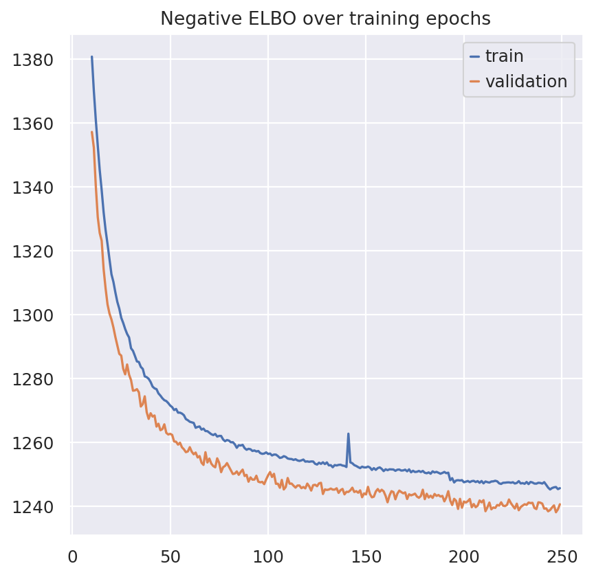
plt.plot(model.history["elbo_train"].iloc[10:], label="train")
plt.plot(model.history["elbo_validation"].iloc[10:], label="validation")
plt.title("Negative ELBO over training epochs")
plt.legend()
<matplotlib.legend.Legend at 0x7f1ff9e52ad0>
TOTALVI_LATENT_KEY = "X_totalvi"

adata.obsm[TOTALVI_LATENT_KEY] = model.get_latent_representation()
Train a classifier on the latent space#
The representation of the reference data will not change when the model gets updated with query data. Therefore, we can train any simple classifier on the latent space. Here we use a Random Forest from scikit-learn.
By storing the classifier object in our totalVI instance (and giving it an attribute that ends with _), we can automatically save and load this classifier along with our model.
y_train = adata.obs["celltype.l2"].astype("category").cat.codes.to_numpy()
X_train = adata.obsm[TOTALVI_LATENT_KEY]
clf = RandomForestClassifier(
    random_state=1,
    class_weight="balanced_subsample",
    verbose=1,
    n_jobs=-1,
)
clf.fit(X_train, y_train)

model.latent_space_classifer_ = clf
Inspect reference model#
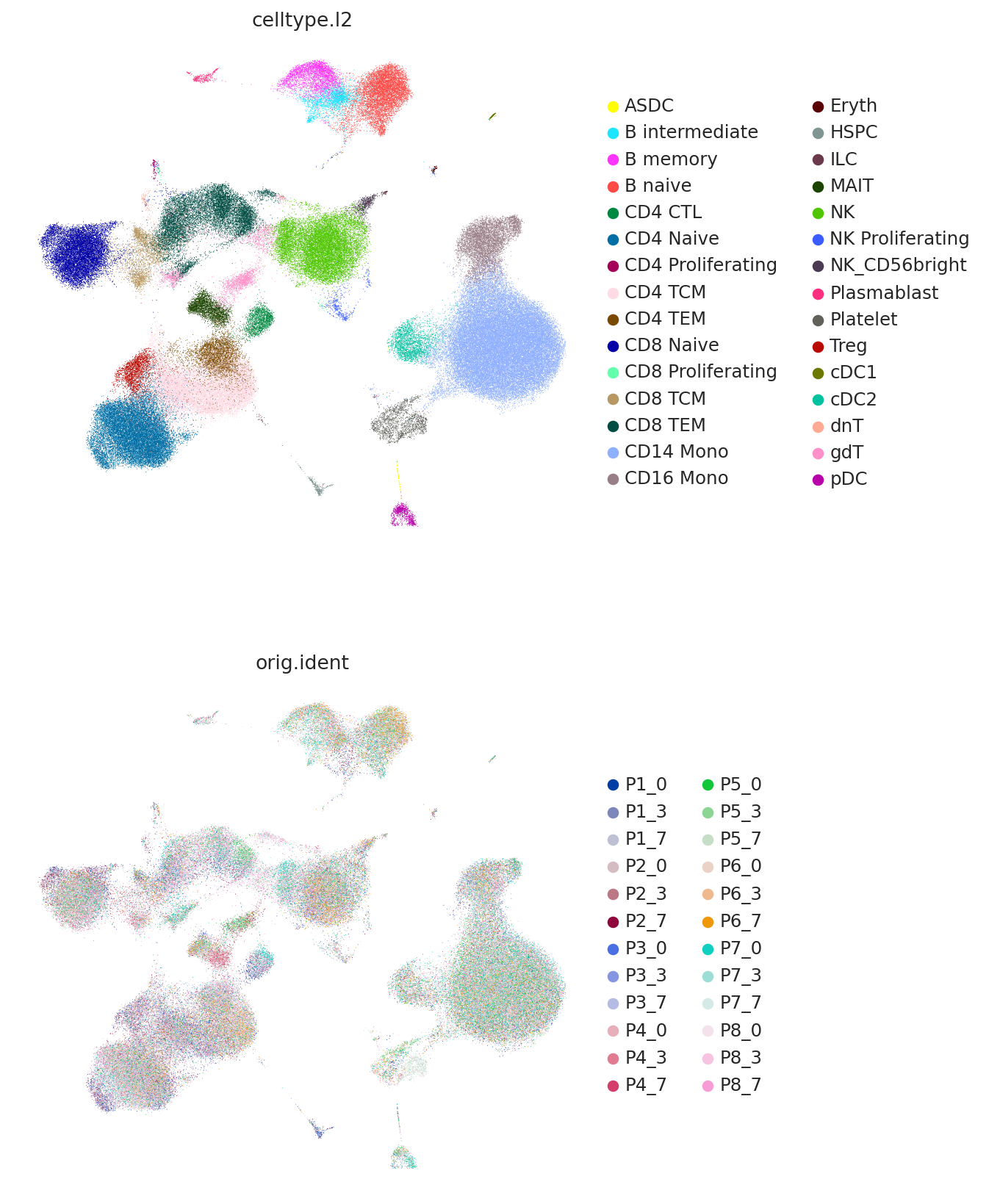
We can view the latent space using UMAP and plot the study-derived cell type labels.
Here we use the umap API instead of scanpy so that we can later use the same umap object on the query data.
TOTALVI_UMAP_KEY = "X_umap"

X = adata.obsm[TOTALVI_LATENT_KEY]
trans = umap.UMAP(
    n_neighbors=10,
    random_state=42,
    min_dist=0.4,
)
adata.obsm[TOTALVI_UMAP_KEY] = trans.fit_transform(X)

model.umap_op_ = trans
sc.pl.umap(
    adata,
    color=["celltype.l2", "orig.ident"],
    frameon=False,
    ncols=1,
)
Map query data#
Now we download our query data and cover the preprocessing necessary to map with our reference model.
In this case our query data are also PBMCs and come from the following study:
Arunachalam, Prabhu S., et al. “Systems biological assessment of immunity to mild versus severe COVID-19 infection in humans.” Science 369.6508 (2020): 1210-1220.
This dataset is also CITE-seq, but contains a subset of the proteins of the reference data.
query_path = os.path.join(save_dir.name, "covid_cite.h5ad")

query = sc.read(
    query_path, backup_url="https://ndownloader.figshare.com/files/27458837"
)
Preprocessing#
First we remove any doublets from the query dataset using Scrublet. This has to be run per batch, which in this dataset is denoted with "set".
query.obs["doublet_scores"] = 0
query.obs["predicted_doublets"] = True
for s in np.unique(query.obs["set"]):
    mask = query.obs["set"] == s
    counts_matrix = query[mask].X.copy()
    scrub = scr.Scrublet(counts_matrix)
    doublet_scores, predicted_doublets = scrub.scrub_doublets()
    query.obs["doublet_scores"].iloc[mask] = doublet_scores
    query.obs["predicted_doublets"].iloc[mask] = predicted_doublets
Preprocessing...
Simulating doublets...
Embedding transcriptomes using PCA...
Calculating doublet scores...
Automatically set threshold at doublet score = 0.37
Detected doublet rate = 3.6%
Estimated detectable doublet fraction = 40.3%
Overall doublet rate:
	Expected   = 10.0%
	Estimated  = 8.9%
Elapsed time: 33.0 seconds
Preprocessing...
Simulating doublets...
Embedding transcriptomes using PCA...
Calculating doublet scores...
Automatically set threshold at doublet score = 0.25
Detected doublet rate = 6.2%
Estimated detectable doublet fraction = 56.4%
Overall doublet rate:
	Expected   = 10.0%
	Estimated  = 11.0%
Elapsed time: 35.9 seconds
Next we do the following:
Store the counts in a layer, perform standard preprocessing
Add blank metadata that we will later fill in with predicted labels
Rename the batch key to correspond to the reference data
Add proteins with all 0 counts for the missing proteins in this query dataset
query.layers["counts"] = query.X.copy()
sc.pp.normalize_total(query, target_sum=1e4)
sc.pp.log1p(query)
query.raw = query
# subset to reference vars
query = query[:, adata.var_names].copy()

query.obsm["protein_counts"] = query.obsm["pro_exp"].copy()
query.obs["celltype.l2"] = "Unknown"
query.obs["orig.ident"] = query.obs["set"]
query.obsm["X_umap"] = query.obs[["UMAP1", "UMAP2"]].values

# reorganize query proteins, missing proteins become all 0
for p in adata.obsm["protein_counts"].columns:
    if p not in query.obsm["protein_counts"].columns:
        query.obsm["protein_counts"][p] = 0.0
# ensure columns are in same order
query.obsm["protein_counts"] = query.obsm["protein_counts"].loc[
    :, adata.obsm["protein_counts"].columns
]
For later visualization, we add some metadata to denote whether the dataset is reference of query
adata.obs["dataset_name"] = "Reference"
query.obs["dataset_name"] = "Query"
Query model training#
query_model = TOTALVI.load_query_data(query, model)
query_model.train(
    max_epochs=150,
    plan_kwargs={"weight_decay": 0.0, "scale_adversarial_loss": 0.0},
)
INFO     Found batches with missing protein expression
INFO     Computing empirical prior initialization for protein background.
Epoch 150/150: 100%|██████████| 150/150 [08:01<00:00,  3.21s/it, v_num=1, train_loss_step=1.07e+3, train_loss_epoch=1.07e+3]
And now we retrieve the latent representation for the query data
TOTALVI_QUERY_LATENT_KEY = "X_totalvi_scarches"

query.obsm[TOTALVI_QUERY_LATENT_KEY] = query_model.get_latent_representation(query)
Query cell type prediction#
We can use the random forest that we previously trained using the latent representation of the query data in the updated model!
# predict cell types of query
predictions = query_model.latent_space_classifer_.predict(
    query.obsm[TOTALVI_QUERY_LATENT_KEY]
)
categories = adata.obs["celltype.l2"].astype("category").cat.categories
cat_preds = [categories[i] for i in predictions]
query.obs["celltype.l2"] = cat_preds
query.obs["predicted_l2_scarches"] = cat_preds
Evaluate label transfer#
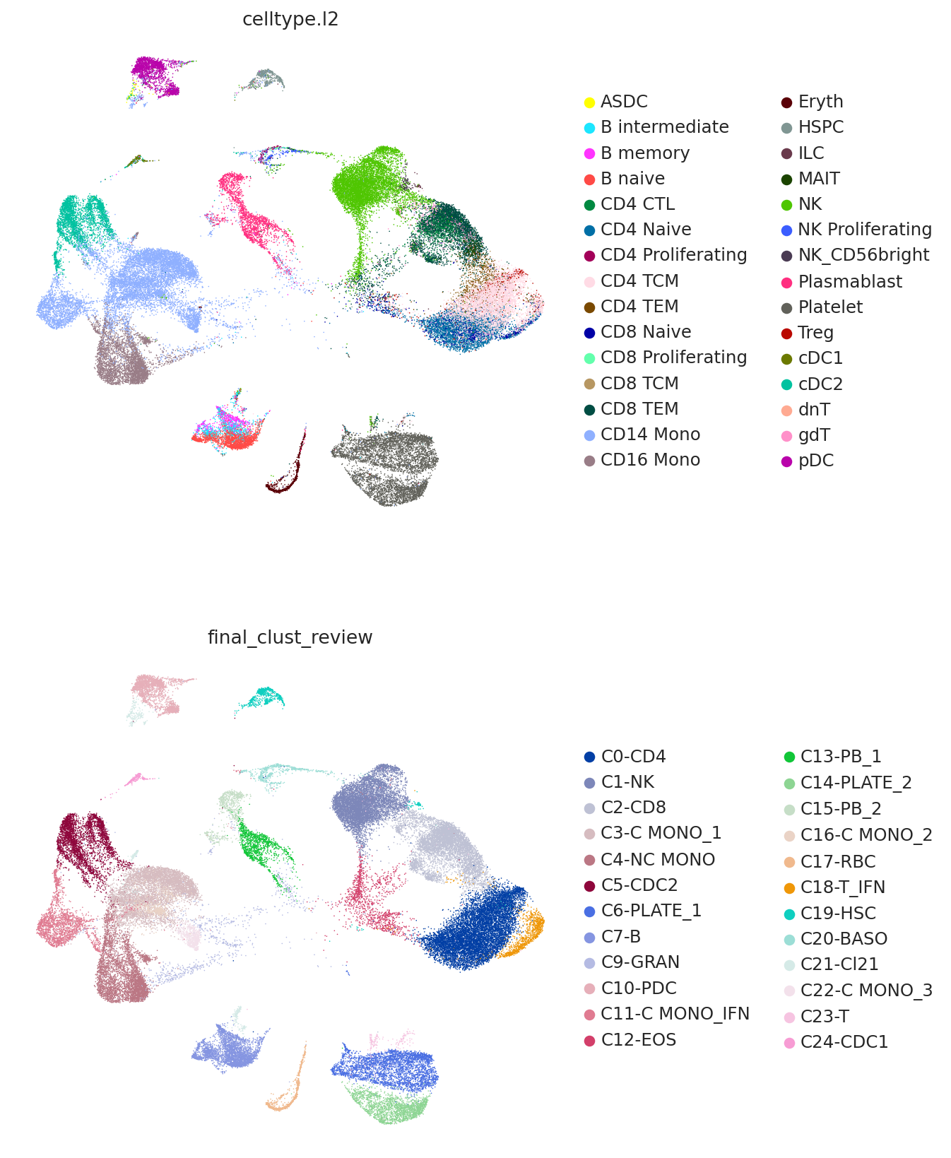
Now we plot the predicted labels and the labels from the query study (here denoted as "final_clust_review") on the UMAP coordinated used in the query study. We can see that we have an overall strong concordance, but also some important differences. For example, the study found a population of monocytes with interferon signaling, but as the reference contains no such cell type, it can only predict them to be CD14 monocytes.
sc.pl.umap(
    query,
    color=["celltype.l2", "final_clust_review"],
    frameon=False,
    ncols=1,
)
Use reference UMAP#
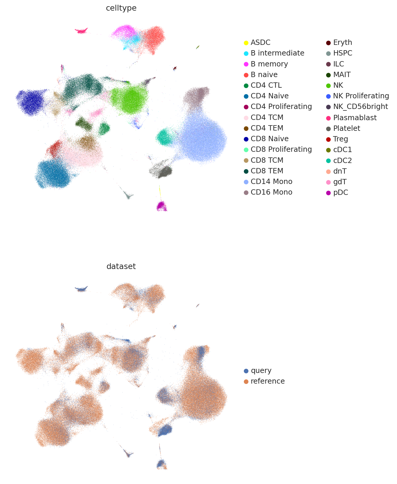
We can also use the same UMAP operator from the reference step to visualize our query data.
TOTALVI_UMAP_PROJECT_KEY = "X_umap_project"

query.obsm[TOTALVI_UMAP_PROJECT_KEY] = query_model.umap_op_.transform(
    query.obsm[TOTALVI_QUERY_LATENT_KEY]
)
sc.pl.embedding(
    query,
    TOTALVI_UMAP_PROJECT_KEY,
    color=["celltype.l2", "final_clust_review"],
    frameon=False,
    ncols=1,
)
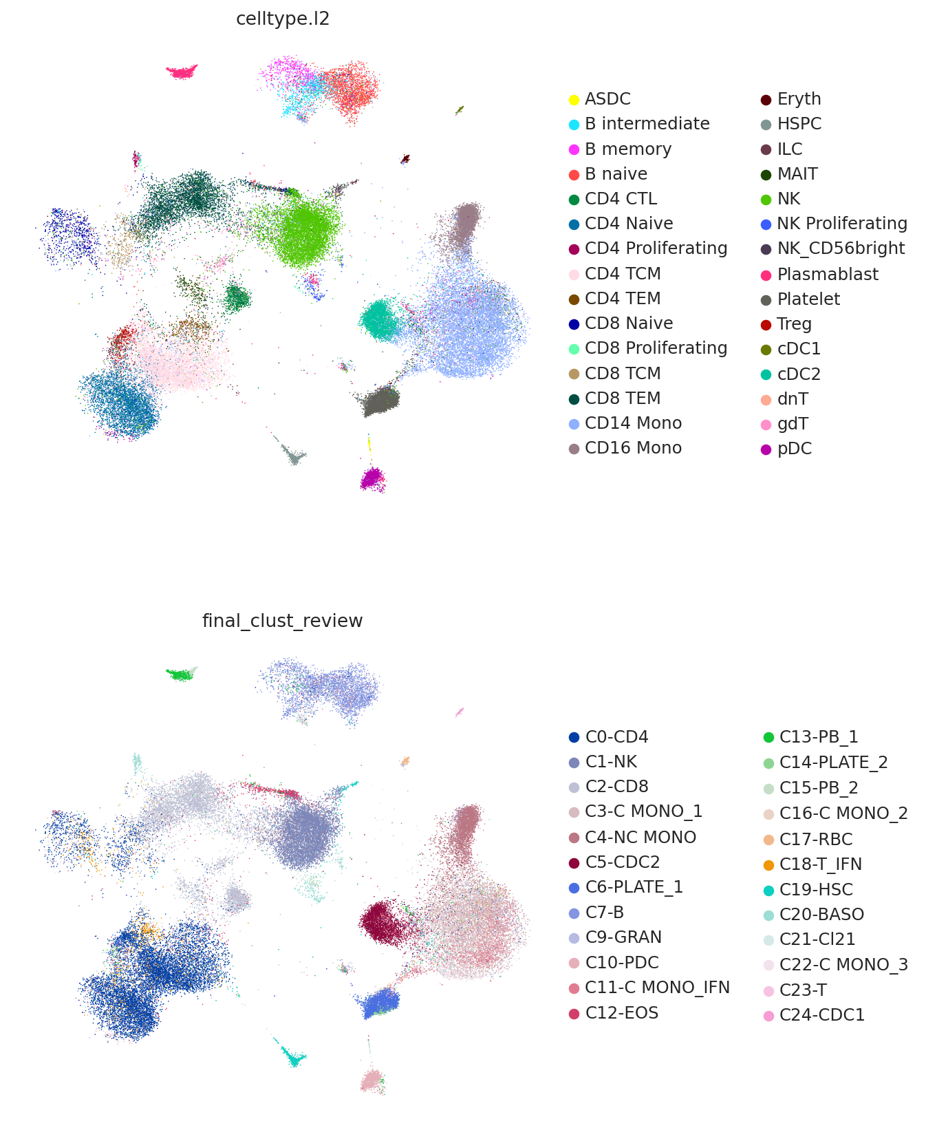
And finally we can combine the umaps together and visualize jointly.
umap_adata = sc.AnnData(
    np.concatenate(
        [
            query.obsm["X_umap_project"],
            adata.obsm["X_umap"],
        ],
        axis=0,
    )
)
umap_adata.obs["celltype"] = np.concatenate(
    [query.obs["celltype.l2"].values, adata.obs["celltype.l2"].values]
)
umap_adata.obs["dataset"] = np.concatenate(
    [query.shape[0] * ["query"], adata.shape[0] * ["reference"]]
)
umap_adata.obsm["X_umap"] = umap_adata.X
inds = np.random.permutation(np.arange(umap_adata.shape[0]))
sc.pl.umap(
    umap_adata[inds],
    color=["celltype", "dataset"],
    frameon=False,
    ncols=1,
)
