Differential expression on C. elegans data

This notebook was contributed by Eduardo Beltrame @Munfred and edited by Romain Lopez, Adam Gayoso, and Pierre Boyeau.

Processing and visualizing 89k cells from Packer et al. 2019 C. elegans 10xv2 single cell data

Original article: A lineage-resolved molecular atlas of C. elegans embryogenesis at single-cell resolution

https://science.sciencemag.org/content/365/6459/eaax1971.long

The anndata object we provide has 89,701 cells and 20,222 genes. It includes short gene descriptions from WormBase that will show up when mousing over the interactive plots.

Steps performed:

1. Loading the data from anndata containing cell labels and gene descriptions

2. Training the model with batch labels for integration with scVI

3. Retrieving the scVI latent space and imputed values

4. Visualize the latent space with an interactive t-SNE plot using Plotly

5. Perform differential expression and visualize with interactive volcano plot and heatmap using Plotly

This notebook was designed to be run in Google Colab.

Note

Running the following cell will install tutorial dependencies on Google Colab only. It will have no effect on environments other than Google Colab.

!pip install --quiet scvi-colab
from scvi_colab import install

install()

WARNING: Running pip as the 'root' user can result in broken permissions and conflicting behaviour with the system package manager. It is recommended to use a virtual environment instead: https://pip.pypa.io/warnings/venv

import os
import tempfile

import matplotlib.pyplot as plt
import numpy as np
import pandas as pd
import plotnine as p9
import scanpy as sc
import scvi
import seaborn as sns
import torch

scvi.settings.seed = 0
print("Last run with scvi-tools version:", scvi.__version__)

Last run with scvi-tools version: 1.1.0

Note

You can modify save_dir below to change where the data files for this tutorial are saved.

sc.set_figure_params(figsize=(6, 6), frameon=False)
sns.set_theme()
torch.set_float32_matmul_precision("high")
save_dir = tempfile.TemporaryDirectory()

%config InlineBackend.print_figure_kwargs={"facecolor": "w"}
%config InlineBackend.figure_format="retina"

adata_path = os.path.join(save_dir.name, "packer2019.h5ad")

adata = sc.read(
    adata_path,
    backup_url="https://github.com/Munfred/wormcells-site/releases/download/packer2019/packer2019.h5ad",
)
adata

AnnData object with n_obs × n_vars = 89701 × 20222
    obs: 'cell', 'numi', 'time_point', 'batch', 'size_factor', 'cell_type', 'cell_subtype', 'plot_cell_type', 'raw_embryo_time', 'embryo_time', 'embryo_time_bin', 'raw_embryo_time_bin', 'lineage', 'passed_qc'
    var: 'gene_id', 'gene_name', 'gene_description'

Take a look at the gene descriptions

The gene descriptions were taken using the WormBase API.

display(
    adata.var.head().style.set_properties(
        subset=["gene_description"], **{"width": "600px"}
    )
)

	gene_id	gene_name	gene_description
index
WBGene00010957	WBGene00010957	nduo-6	Is affected by several genes including daf-16; daf-12; and hsf-1 based on RNA-seq and tiling array studies. Is affected by six chemicals including Rotenone; Psoralens; and metformin based on RNA-seq and microarray studies.
WBGene00010958	WBGene00010958	ndfl-4	Is enriched in Psub2 based on RNA-seq studies. Is affected by several genes including daf-16; daf-12; and clk-1 based on RNA-seq and microarray studies. Is affected by six chemicals including Alovudine; Psoralens; and metformin based on RNA-seq studies.
WBGene00010959	WBGene00010959	nduo-1	Is an ortholog of human MT-ND1 (mitochondrially encoded NADH:ubiquinone oxidoreductase core subunit 1). Is predicted to contribute to NADH dehydrogenase activity. Human ortholog(s) of this gene are implicated in Leber hereditary optic neuropathy and MELAS syndrome.
WBGene00010960	WBGene00010960	atp-6	Is predicted to contribute to proton-transporting ATP synthase activity, rotational mechanism.
WBGene00010961	WBGene00010961	nduo-2	Is affected by several genes including hsf-1; clk-1; and elt-2 based on RNA-seq and microarray studies. Is affected by eight chemicals including stavudine; Zidovudine; and Psoralens based on RNA-seq and microarray studies.

Selecting genes and loading data

We use the utility scvi.data.poisson_gene_selection to select genes according to their dropout rate, which is a simple and scalable approach to select genes.

This method was described by Andrews & Hemberg in the article M3Drop: dropout-based feature selection for scRNASeq : https://academic.oup.com/bioinformatics/article/35/16/2865/5258099

This method modifies the adata to add the following fields:

highly_variable                   # boolean true for chosen genes
observed_fraction_zeros	       # fraction of observed zeros per gene
expected_fraction_zeros	       # expected fraction of observed zeros per gene
prob_zero_enriched_nbatches	   # If batch_key is given, this denotes in how many batches genes are detected as zero enriched
prob_zero_enrichment	          # Probability of zero enrichment, median across batches in the case of multiple batches
prob_zero_enrichment_rank         # Rank of the gene according to probability of zero enrichment

Note

Gene selection is an important step to obtain relevant cell representations with scVI. Generally, selecting the top few thousands top-ranking genes predicted by a gene selection tool suffice to obtain good performance.

Increasing the number of selected genes may be required in some applications, e.g., to increase the number of considered genes for differential expression. Note, however, that this will increase the time required to reach convergence and GPU memory load. It may also require to tune scVI’s model hyperparameters (see the autotune tutorial)

Alternatives to the Poisson gene selection can be used, e.g., via scanpy or seurat.

scvi.data.poisson_gene_selection(adata)
adata.var.head()

Sampling from binomial...: 100%|██████████| 10000/10000 [00:00<00:00, 21246.35it/s]

	gene_id	gene_name	gene_description	highly_variable	observed_fraction_zeros	expected_fraction_zeros	prob_zero_enriched_nbatches	prob_zero_enrichment	prob_zero_enrichment_rank
index
WBGene00010957	WBGene00010957	nduo-6	Is affected by several genes including daf-16;...	False	0.075685	0.002028	0	0.0762	15661.0
WBGene00010958	WBGene00010958	ndfl-4	Is enriched in Psub2 based on RNA-seq studies....	True	0.659680	0.623356	1	0.2502	19567.0
WBGene00010959	WBGene00010959	nduo-1	Is an ortholog of human MT-ND1 (mitochondriall...	True	0.201993	0.046608	1	0.1886	18907.0
WBGene00010960	WBGene00010960	atp-6	Is predicted to contribute to proton-transport...	True	0.138081	0.001848	1	0.1381	17859.0
WBGene00010961	WBGene00010961	nduo-2	Is affected by several genes including hsf-1; ...	True	0.468434	0.383116	1	0.2860	19800.0

adata = adata[:, adata.var["highly_variable"]]  # focus on selected genes
adata.layers[
    "counts"
] = adata.X.copy().tocsr()  # converts to CSR format, preserve counts

scvi.model.SCVI.setup_anndata(
    adata, layer="counts", batch_key="batch"
)  # prepare data for scVI

Define and train the model

model = scvi.model.SCVI(
    adata, gene_likelihood="nb"
)  # We use Negative Binomial count likelihoods, following Boyeau et al., 2023.
model.train(
    check_val_every_n_epoch=1,
    max_epochs=400,
    early_stopping=True,
    early_stopping_patience=20,
    early_stopping_monitor="elbo_validation",
)

Epoch 400/400: 100%|██████████| 400/400 [20:15<00:00,  3.04s/it, v_num=1, train_loss_step=2.03e+3, train_loss_epoch=2.06e+3]

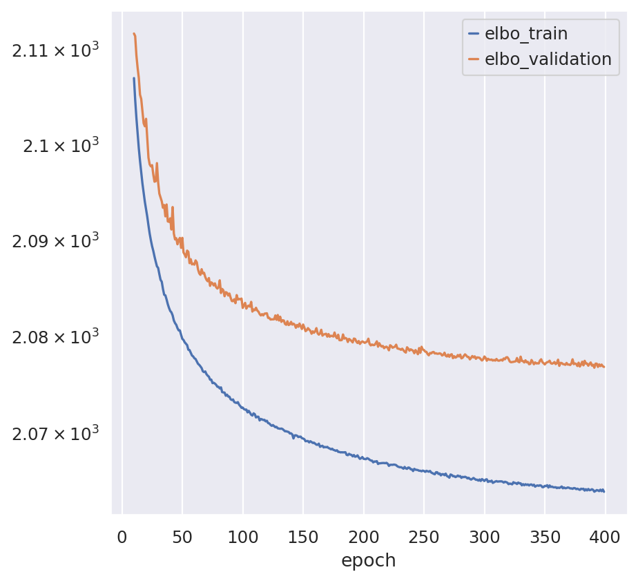
# Ensure convergence
train_test_results = model.history["elbo_train"]
train_test_results["elbo_validation"] = model.history["elbo_validation"]
train_test_results.iloc[10:].plot(logy=True)  # exclude first 10 epochs
plt.show()

Get the latent space and compute UMAP

SCVI_LATENT_KEY = "X_scVI"

latent = model.get_latent_representation()
adata.obsm[SCVI_LATENT_KEY] = latent
sc.pp.neighbors(adata, use_rep=SCVI_LATENT_KEY)
sc.tl.umap(adata)
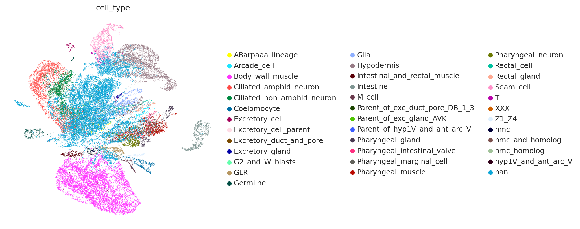
sc.pl.umap(adata, color="cell_type")

Performing Differential Expression in scVI

Differential expression (DE) analysis is used to quantify the differences in gene expression across subpopulations of genes. If we have two sets of cells \(A\) and \(B\), a DE test is typically used to predict two things for each gene:

1. Whether the gene’s expression levels are significantly different in the A and B sets of cells.

2. An effect size that quantifies the strength of the differential expression.

Once trained, scVI can natively perform both of these tasks. Additionally, its differential expression module can account for batch effects and filter DE genes expected to be of little relevance.

Selecting cell subpopulations to compare

# let's take a look at abundances of different cell types
adata.obs["cell_type"].value_counts()

cell_type
nan                               35052
Body_wall_muscle                  17520
Hypodermis                         7746
Ciliated_amphid_neuron             6090
Ciliated_non_amphid_neuron         4468
Seam_cell                          2766
Pharyngeal_muscle                  2562
Glia                               1857
Intestine                          1732
Pharyngeal_neuron                  1471
Pharyngeal_marginal_cell            911
Coelomocyte                         787
Pharyngeal_gland                    786
GLR                                 768
Intestinal_and_rectal_muscle        568
Germline                            499
Pharyngeal_intestinal_valve         493
Arcade_cell                         434
Z1_Z4                               372
Rectal_cell                         327
M_cell                              315
ABarpaaa_lineage                    273
Rectal_gland                        265
Excretory_cell                      215
Excretory_gland                     205
hmc                                 189
hmc_homolog                         155
T                                   141
hmc_and_homolog                     122
Parent_of_exc_gland_AVK             114
hyp1V_and_ant_arc_V                 112
Excretory_duct_and_pore              91
Parent_of_hyp1V_and_ant_arc_V        75
G2_and_W_blasts                      72
Excretory_cell_parent                62
Parent_of_exc_duct_pore_DB_1_3       61
XXX                                  25
Name: count, dtype: int64

scVI provides several options to identify the two populations of interest.

cell_type_1 = "Ciliated_non_amphid_neuron"
cell_idx1 = adata.obs["cell_type"] == cell_type_1
print(sum(cell_idx1), "cells of type", cell_type_1)

cell_type_2 = "Intestine"
cell_idx2 = adata.obs["cell_type"] == cell_type_2
print(sum(cell_idx2), "cells of type", cell_type_2)

# or equivalently, provide a string of the form "my_celltype_column == 'desired_celltype'"
# cell_idx1 = "cell_type == 'Ciliated_non_amphid_neuron'"
# cell_idx2 = "cell_type == 'Intestine'"

4468 cells of type Ciliated_non_amphid_neuron
1732 cells of type Intestine

Basic principle

DE and log fold-changes

scVI can natively be used to perform differential expression analyses to compare populations of cells, as described here and there. It achieves this by estimating the posterior distribution of the log fold-change (LFC) between subpopulations \(A\) and \(B\). Specifically, for a given gene g, scVI calculates the LFC as the difference between the logarithm of its expression level in population A, denoted by \(h_g^A\), and the logarithm of its expression level in population B, denoted by \(h_g^B\).

The resulting value, denoted by \(\beta_g\), provides insights into the expression patterns of gene \(g\). Values close to zero indicate that the gene is expressed similarly in both populations, positive values suggest upregulation in population A and negative values indicate downregulation in population A. This information can be used to better understand the biological mechanisms underlying the differences between the two cell populations.

DE testing

In addition to estimating the LFC, scVI can also detect which genes have significant expression patterns. To tag which genes are differentially expressed, scVI tests the following competing hypotheses \(M_{1, g}: \beta_g \in [-\delta, \delta]\) and \(M_{2, g}: \beta_g \in (-\infty, -\delta) \cup (\delta, \infty)\). Here, \(\delta\) denotes a small LFC threshold, such that \(\beta_g \in [-\delta, \delta]\) is evidence that the gene is equally expressed in the two subpopulations.

Differentially expressed genes are identified by computing the posterior probability of \(M_{2, g}\).

Running DE analyses

Running and understanding a DE run

A simple DE analysis can then be performed using the following command

de_change = model.differential_expression(idx1=cell_idx1, idx2=cell_idx2)
de_change

DE...: 100%|██████████| 1/1 [00:00<00:00,  1.20it/s]

	proba_de	proba_not_de	bayes_factor	scale1	scale2	pseudocounts	delta	lfc_mean	lfc_median	lfc_std	lfc_min	lfc_max	raw_mean1	raw_mean2	non_zeros_proportion1	non_zeros_proportion2	raw_normalized_mean1	raw_normalized_mean2	is_de_fdr_0.05
index
WBGene00006870	1.0000	0.0000	18.420681	0.000400	0.000004	0.0	0.25	7.165903	7.197666	1.520534	-1.765389	12.305556	0.567147	0.028291	0.252686	0.025982	5.500196	0.044442	True
WBGene00011938	1.0000	0.0000	18.420681	0.000013	0.000480	0.0	0.25	-5.446735	-5.540369	1.405468	-9.422789	1.125211	0.011638	3.357980	0.010072	0.834873	0.128841	4.526570	True
WBGene00013560	0.9998	0.0002	8.516943	0.000038	0.001268	0.0	0.25	-4.677629	-4.729869	1.584986	-9.786007	2.483212	0.035586	8.210736	0.030886	0.898961	0.340279	12.123684	True
WBGene00011121	0.9998	0.0002	8.516943	0.001431	0.000006	0.0	0.25	7.113941	7.609168	2.303849	-1.747072	12.854574	1.442006	0.040416	0.537601	0.038684	14.994382	0.059873	True
WBGene00000452	0.9998	0.0002	8.516943	0.000240	0.000005	0.0	0.25	5.858909	5.913099	1.573072	-1.599674	11.946387	0.376680	0.033487	0.123545	0.027136	3.191612	0.074427	True
...	...	...	...	...	...	...	...	...	...	...	...	...	...	...	...	...	...	...	...
WBGene00022044	0.5808	0.4192	0.326058	0.000182	0.000167	0.0	0.25	0.164114	0.127701	0.512683	-1.325256	3.128280	0.189124	1.164550	0.163608	0.618938	1.599760	1.586375	False
WBGene00044608	0.5746	0.4254	0.300644	0.000109	0.000094	0.0	0.25	0.215397	0.201292	0.418493	-1.350334	2.464341	0.146599	0.693418	0.123545	0.452079	1.315090	0.948504	False
WBGene00022702	0.5600	0.4400	0.241162	0.000062	0.000062	0.0	0.25	0.000142	-0.035827	0.532482	-1.729041	3.303222	0.075649	0.457272	0.068039	0.340647	0.639998	0.621169	False
WBGene00011116	0.5184	0.4816	0.073633	0.000302	0.000267	0.0	0.25	0.175932	0.171164	0.354389	-1.125929	1.881635	0.356761	1.845267	0.275067	0.763279	2.979073	2.603784	False
WBGene00011859	0.4998	0.5002	-0.000800	0.000122	0.000115	0.0	0.25	0.099528	0.064282	0.494328	-1.683570	3.587107	0.141899	0.824482	0.122426	0.515589	1.178068	1.153656	False

4000 rows × 19 columns

This method returns a pandas DataFrame, where each row corresponds to a gene. The most important columns of this dataframe are the following. proba_de, which captures the posterior probability of \(M_{2, g}\) that the gene is differentially expressed. Values close to one indicate that the gene is DE; lfc_mean and lfc_median, respectively denoting the mean and the median of the posterior distribution of \(\beta_g\). Positive values of the LFC signify that the gene is upregulated in idx1; is_de_fdr_0.05 is True when the gene is tagged DE after FDR correction at target level \(\alpha=0.05\). The target level can be adjusted by specifying fdr_target in the differential_expression method.

Main hyperparameters

Additional parameters can be tuned in specific applications.

1. weights, which can correspond to ”uniform” or ”importance” specify how normalized gene expressions in the two subpopulations are computed. The ”importance” flavor is specifically designed to provide FDR-calibrated gene sets, but may be overkill if you only aim to rank genes (via their LFC for instance).

2. filter_outlier_cells filters out outlier cells prior to computing normalized gene expressions. It is important to set this parameter to True when weights='importance'.

3. delta allows to specify \(\delta\), which is used to detect differentially expressed genes. It can also be set automatically using delta=None

4. pseudocounts, which is zero by default, but can be set to a small value (e.g., 1e-6) when many detected DE genes are seldom expressed in the compared populations.

5. batch_correction, which should be set to True to account for batch effects. This only makes sense when idx1 and idx2 denote cells coming from overlapping batches.

The exact function of these parameters is described here.

Volcano plot of change mode DE with p-values

de_change_uniform = model.differential_expression(
    idx1=cell_idx1,  # we use the same cells as chosen before
    idx2=cell_idx2,
    weights="uniform",
    batch_correction=True,
)

# manipulate the DE results for plotting
de_change_uniform["log10_pscore"] = np.log10(de_change_uniform["proba_not_de"])
de_change_uniform = de_change_uniform.join(adata.var, how="inner")
de_change_uniform.head()

DE...: 100%|██████████| 1/1 [00:01<00:00,  1.54s/it]

	proba_de	proba_not_de	bayes_factor	scale1	scale2	pseudocounts	delta	lfc_mean	lfc_median	lfc_std	...	log10_pscore	gene_id	gene_name	gene_description	highly_variable	observed_fraction_zeros	expected_fraction_zeros	prob_zero_enriched_nbatches	prob_zero_enrichment	prob_zero_enrichment_rank
index
WBGene00018727	1.0000	0.0000	18.420681	0.001506	0.000004	0.0	0.25	8.083410	8.553434	2.452872	...	-inf	WBGene00018727	jbts-14	Is involved in non-motile cilium assembly. Loc...	True	0.923044	0.843094	1	0.1451	18051.0
WBGene00004372	1.0000	0.0000	18.420681	0.000978	0.000005	0.0	0.25	7.747259	7.895372	1.346017	...	-inf	WBGene00004372	rig-5	Is an ortholog of human LSAMP (limbic system a...	True	0.928574	0.814163	1	0.1740	18667.0
WBGene00007266	1.0000	0.0000	18.420681	0.000556	0.000012	0.0	0.25	5.491581	5.608122	1.399333	...	-inf	WBGene00007266	C03A3.1	Is enriched in nervous system and pharynx base...	True	0.714697	0.654044	1	0.2390	19470.0
WBGene00007119	1.0000	0.0000	18.420681	0.000597	0.000009	0.0	0.25	5.797742	5.903028	1.622160	...	-inf	WBGene00007119	calf-1	Is involved in several processes, including de...	True	0.832276	0.797743	1	0.1644	18475.0
WBGene00043097	0.9998	0.0002	8.516543	0.000014	0.000153	0.0	0.25	-3.516246	-3.542899	0.972021	...	-3.698796	WBGene00043097	C02D5.4	Is an ortholog of human GSTO1 (glutathione S-t...	True	0.919165	0.881716	1	0.1124	17138.0

5 rows × 29 columns

de_change_importance = model.differential_expression(
    idx1=cell_idx1,  # we use the same cells as chosen before
    idx2=cell_idx2,
    weights="importance",
    filter_outlier_cells=True,
    batch_correction=True,
)

# manipulate the DE results for plotting
de_change_importance["log10_pscore"] = np.log10(de_change_importance["proba_not_de"])
de_change_importance = de_change_importance.join(adata.var, how="inner")

DE...: 100%|██████████| 1/1 [00:52<00:00, 52.94s/it]

de_comp = pd.concat(
    [
        de_change_importance.assign(flavor="importance"),
        de_change_uniform.assign(flavor="uniform"),
    ]
)
de_comp["gene_type"] = "Other"
de_comp.loc[lambda x: x["gene_name"].str.contains("rpl-"), "gene_type"] = "RPL"
de_comp.loc[lambda x: x["gene_name"].str.contains("ceh-"), "gene_type"] = "CEH"
de_comp.loc[lambda x: x["gene_name"].str.contains("flp-"), "gene_type"] = "FPL"

(
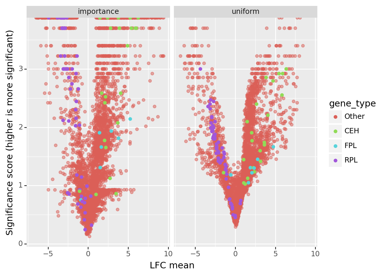
    p9.ggplot(de_comp, p9.aes("lfc_mean", "-log10_pscore", color="gene_type"))
    + p9.geom_point(
        de_comp.query("gene_type == 'Other'"), alpha=0.5
    )  # Plot other genes with transparence
    + p9.geom_point(de_comp.query("gene_type != 'Other'"))
    + p9.labs(x="LFC mean", y="Significance score (higher is more significant)")
    + p9.facet_wrap("flavor")
)

<Figure Size: (640 x 480)>

Contrary to the uniform flavor, the importance flavor returns sharper posterior probability scores (posterior probability near 0 or 1, respectively in case of equal expression or differential expression).

Heatmap of top expressed genes

Now we perform DE between each cell type vs all other cells and make a heatmap of the result.

# here we do a 1-vs-all DE test, which compares each cell type with all others
# this returns the concatenation of all 1vsall results, contained in a DataFrame
change_per_cluster_de = model.differential_expression(groupby="cell_type")

DE...: 100%|██████████| 37/37 [02:21<00:00,  3.82s/it]

We focus on cell-types with at least 500 cells, and which have annotations to facilitate heatmap visualization

cell_types = (
    adata.obs["cell_type"]
    .value_counts()
    # .loc[lambda x: (x >= 500) & (x.index != "nan")]
    .loc[lambda x: x.index != "nan"]
    .to_frame("n_cells")
)
cell_types.loc[:, "associated_test"] = cell_types.index.astype(str) + " vs Rest"

# This cell extracts list of top 5 upregulated genes for every cell-type
marker_genes = (
    change_per_cluster_de.reset_index()
    .loc[lambda x: x.comparison.isin(cell_types.associated_test.values)]
    .groupby("comparison")
    .apply(
        lambda x: x.sort_values("lfc_mean", ascending=False).iloc[:5]
    )  # Select top 5 DE genes per comparison
    .reset_index(drop=True)["index"]
    .unique()
)

adata_log = adata[adata.obs.cell_type.isin(cell_types.index.values)].copy()
sc.pp.normalize_total(adata_log)
sc.pp.log1p(adata_log)
sc.pl.dotplot(adata_log, marker_genes, groupby="cell_type")