Integration of scRNA-seq data with substantial batch effects using sysVI

This tutorial shows how to integrate scRNA-seq datasets with substantial batch effects (here referred to as systems), such as cross-species, cross-technology (e.g. cells and nuclei), and primary tissue and in vitro model system (e.g. organoid) datasets. In this tutorial, we use the sysVI model that combines VampPrior and latent cycle-consistency loss on top of a cVAE to improve integration.

For more details on this method please see our paper Integrating single-cell RNA-seq datasets with substantial batch effects.

While sysVI is implemented in Python, users may decide to call it from R via the reticulate package as shown in this scvi-tools tutorial or to convert their data objects between R and Python with packages anndata2ri and zellkonverter to make use of sysVI directly in Python.

!pip install --quiet scvi-colab
from scvi_colab import install

install()

import os
import tempfile

import matplotlib.pyplot as plt
import scanpy as sc

# Reproducibility
import scvi
from scvi.external import SysVI

scvi.settings.seed = 0
print("Last run with scvi-tools version:", scvi.__version__)

Last run with scvi-tools version: 1.3.0

Prepare data for integration

Prepare features

In general, it is important that the feature characteristics match across systems, as this is key for successful integration. For example, if you used the model on scRNA-seq data it needs to be correctly preprocessed, as described below, and similarly, if you tested it on other data types, such as image features, good preprocessing is likewise vital. Furthermore, please keep in mind that the model assumes Gaussian noise distribution of features.

For scRNA-seq data the integration should be performed on normalized and log-transformed data, with normalization being set to a fixed number of counts per cell. We recomend that data should be subsetted to HVGs before integration. In our paper we selected HVGs per system (e.g. species) with Scanpy function pp.highly_variable_genes using within-system batches as the batch_key, starting with genes present in all systems. Then, we took the intersection of HVGs across systems to obtain ~2000 shared HVGs. The here-used example data was already preprocessed accordingly and has normalized data in X.

Prepare covariates

For integration we must define covariates to be corrected for by the model. The batch_key covariate should represent the covariate capturing the substantial batch effects, also referred to as “system” in our publication. Besides system covariate, any other relatively weaker batch effects of a continuous or categorical nature can be corrected for as part of the standard conditioning within cVAE training. This can be for example samples within systems, denoted by obs column “batch” in the below example.

If you have more than one type of system, such as species and technology, you can try to set the system to their combination. For example, if integrating cell and nuclei data from mouse and human the systems should be: mouse-nuclei, mouse-cell, human-nuclei, human-cell. This system grouping should be likewise used for data preprocessing, such as HVG selection.

If the number of categories in additional categorical covariates is extensive, the one-hot encoding would lead to large memory usage. In this case, categorical covariates should be embedded by setting embed_cat = True during Model initialization, as explained below.

# Load data
# Save dir may be changed as desired
save_dir = tempfile.TemporaryDirectory()
adata_path = os.path.join(save_dir.name, "mouse-human_pancreas_subset10000.h5ad")
adata = sc.read(
    adata_path,
    backup_url="https://github.com/theislab/cross_system_integration/raw/main/tutorials/data/mouse-human_pancreas_subset10000.h5ad",
)
adata

AnnData object with n_obs × n_vars = 10000 × 1768
    obs: 'batch', 'mm_study', 'mm_sex', 'mm_age', 'mm_study_sample_design', 'mm_hc_gene_programs_parsed', 'mm_leiden_r1.5_parsed', 'cell_type_eval', 'system', 'hs_Sex', 'hs_Diabetes Status', 'leiden_system'
    var: 'gs_mm', 'gs_hs'
    obsm: 'X_pca_system'
    layers: 'counts'

# Setup adata for training
SysVI.setup_anndata(
    adata=adata,
    batch_key="system",
    categorical_covariate_keys=["batch"],
)

Train the model

To embedd categorical covariates, the model can be initialized with embed_categorical_covariates=True as shown below. This will embed all categorical covariates, including batch_key.

# Example showing how to turn on embedding of all categorical covariates
model = SysVI(
    adata=adata,
    embed_categorical_covariates=True,
)

We suggest that the model with the VampPrior and latent cycle-consistency is used, as shown below. However, if desired, the prior can be changed to standard normal distribution or the number of prior components for VampPrior can be modified during Model initialization. To disable cycle-consistency you can set the z_distance_cycle_weight to zero via plan_kwargs in train, which will then correspond to vanilla cVAE with the chosen prior.

# Example showing how to adjust loss weights
model.train(
    plan_kwargs={
        "kl_weight": 1,
        "z_distance_cycle_weight": 0
        # Add additional parameters, such as number of epochs
    }
)

To increase batch correction you can increase cycle-consistency loss weight and to improve biological preservation you can decrease the KL loss weight or also cycle-consistency loss weight. In a few cases we observed the best integration performance with cycle-consistency loss weight as high as 50, although the range of 2-10 was usually preferred.

The number of epochs can be reduced when using a dataset with more cells. Please inspect the loss plots below to confirm that the number of epochs is sufficient for the loss to stabilize.

Another thing to keep in mind is that model performance may vary depending on the used random seed, as reported in our paper. Thus, it may be beneficial to run a few (e.g. three) models with different random seeds and pick the best one. Random seed for scvi-tools can be set as shown below, before training the model.

# Change the seed
scvi.settings.seed = 1

# Now initialise and train the model
model = SysVI(adata=adata)
model.train()

# Initialise the model
model = SysVI(adata=adata)
# Train
max_epochs = 200
model.train(
    max_epochs=max_epochs, check_val_every_n_epoch=1, plan_kwargs={"z_distance_cycle_weight": 5}
)

INFO     The model has been initialized

Inspect the losses to assess if the training was succesful

Training loss is plotted in blue and validation loss (held out random cells) in orange. The two losses will be similar due to the cells being randomly sampled into training/validation set without any stratification that would create truly distinct training/validation cell populations.

The top row shows the whole training history while the bottom row shows a zoom-in into the epochs at the end of the training.

# Plot loses
# The plotting code below was specifically adapted to the above-specified model and its training
# If changing the model or training the plotting functions may need to be adapted accordingly

# Make detailed plot after N epochs
epochs_detail_plot = 100

# Losses to plot
losses = [
    "reconstruction_loss_train",
    "kl_local_train",
    "cycle_loss_train",
]
fig, axs = plt.subplots(2, len(losses), figsize=(len(losses) * 3, 4))
for ax_i, l_train in enumerate(losses):
    l_val = l_train.replace("_train", "_validation")
    l_name = l_train.replace("_train", "")
    # Change idx of epochs to start with 1
    l_val_values = model.trainer.logger.history[l_val].copy()
    l_val_values.index = l_val_values.index + 1
    l_train_values = model.trainer.logger.history[l_train].copy()
    l_train_values.index = l_train_values.index + 1
    for l_values, c, alpha, dp in [
        (l_train_values, "tab:blue", 1, epochs_detail_plot),
        (l_val_values, "tab:orange", 0.5, epochs_detail_plot),
    ]:
        axs[0, ax_i].plot(l_values.index, l_values.values.ravel(), c=c, alpha=alpha)
        axs[0, ax_i].set_title(l_name)
        axs[1, ax_i].plot(l_values.index[dp:], l_values.values.ravel()[dp:], c=c, alpha=alpha)

fig.tight_layout()

Integrated embedding

Below we show how to obtain the integrated embedding after the model is trained and visually assess cell type preservation and system integration. For more detailed evaluation examples and integration metrics see our paper.

# Get embedding - save it into X of new AnnData
embed = model.get_latent_representation(adata=adata)
embed = sc.AnnData(embed, obs=adata.obs)
# Make system categorical for plotting below
embed.obs["system"] = embed.obs["system"].map({0: "mouse", 1: "human"})

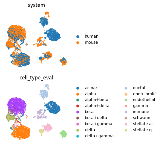
Plot the integrated embedding with system and cell type information to assess the integration quality.

# Compute UMAP
sc.pp.neighbors(embed, use_rep="X")
sc.tl.umap(embed)

# Plot UMAP embedding

# Obs columns to color by
cols = ["system", "cell_type_eval"]

# One plot per obs column used for coloring
fig, axs = plt.subplots(len(cols), 1, figsize=(3, 3 * len(cols)))
for col, ax in zip(cols, axs, strict=False):
    sc.pl.embedding(
        embed,
        "X_umap",
        color=col,
        s=10,
        ax=ax,
        show=False,
        sort_order=False,
        frameon=False,
    )

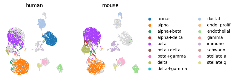
To inspect cell type preservation and system integration in more detail we suggest plotting cell types separately per system.

# Plot UMAP embedding per system
systems = sorted(embed.obs.system.unique())
ncols = len(systems)
# Plot systms side by side
fig, axs = plt.subplots(1, ncols, figsize=(3 * ncols, 3))
for i, system in enumerate(systems):
    ax = axs[i]
    # Plot all cells as background and on top cells from one system colored by cell type
    sc.pl.umap(embed, ax=ax, show=False, s=5, frameon=False)
    sc.pl.umap(
        embed[embed.obs.system == system, :],
        color="cell_type_eval",
        ax=ax,
        show=False,
        s=10,
        frameon=False,
        title=system,
    )
    # Keep legend only on the last plot (assuming this legend contains all categories)
    if i != ncols - 1:
        ax.get_legend().remove()