Differential Expression

Note

This page is under construction.

Problem statement

Differential expression analyses aim to quantify and detect expression differences of some quantity between conditions, e.g., cell types. In single-cell experiments, such quantity can correspond to transcripts, protein expression, or chromatin accessibility. A central notion when comparing expression levels of two cell states is the log fold-change

\begin{align} \beta_g := \log h_{g}^B - \log h_{g}^A, \end{align}

where \(\log h_{g}^A, \log h_{g}^B\) respectively denote the mean expression levels in subpopulations \(A\) and \(B\).

Motivation

In the particular case of single-cell RNA-seq data, existing differential expression models often model that the mean expression level \(\log h_{g}^C\). as a linear function of the cell-state and batch assignments. These models face two notable limitations to detect differences in expression between cell-states in large-scale scRNA-seq datasets. First, such linear assumptions may not capture complex batch effects existing in such datasets accurately. When comparing two given states \(A\) and \(B\) in a large dataset, these models may also struggle to leverage data of a related state present in the data.

Deep generative models may not suffer from these problems. Most scvi-tools models use complex nonlinear mappings to capture batch effects on expression. Using amortization, they can leverage large amounts of data to better capture shared correlations between features. Consequently, deep generative models have appealing properties for differential expression in large-scale data.

This guide has two objectives. First, it aims to provide insight as to how scVI-tools’ differential expression module works for transcript expression (scVI), surface protein expression (TOTALVI), or chromatin accessibility (PeakVI). More precisely, we explain how it can:

• approximate population-specific normalized expression levels

• detect biologically relevant features

• provide easy-to-interpret predictions

More importantly, this guide explains the function of the hyperparameters of the differential_expression method.

Parameter	Description	Approximating expression levels	Detecting relevant features	Providing easy-to-interpret predictions
idx1, idx2	Mask or queries for the compared populations \(A\) and \(B\).	yes
mode	Characterizes the null hypothesis.		yes
delta	composite hypothesis characteristics (when mode="change").		yes
fdr_target	desired FDR significance level			yes
importance_sampling	Precises if expression levels are estimated using importance sampling	yes

Notations and model assumptions

While considering different modalities, scVI, TOTALVI, and PeakVI share similar properties, allowing us to perform differential expression of transcripts, surface proteins, or chromatin accessibility, similarly. We first introduce some notations that will be useful in the remainder of this guide. In particular, we consider a deep generative model where a latent variable with prior \(z_n \sim \mathcal{N}_d(0, I_d)\) represents cell \(n\)’s identity. In turn, a neural network \(f^h_\theta\) maps this low-dimensional representation to normalized, expression levels.

Approximating population-specific normalized expression levels

A first step to characterize differences in expression consists in estimating state-specific expression levels. For several reasons, most scVI-tools models do not explicitly model discrete cell types. A given cell’s state often is unknown in the first place, and inferred with scvi-tools. In some cases, states may also have an intricate structure that would be difficult to model. The class of models we consider here assumes that a latent variable \(z\) characterizes cells’ biological identity. A key component of our differential expression module is to aggregate the information carried by individual cells to estimate population-wide expression levels. The strategy to do so is as follows. First, we estimate latent representations of the two compared states \(A\) and \(B\), using aggregate variational posteriors. In particular, we will represent state \(C\) latent representation with the mixture

\begin{align} \hat P^C( Z ) = \frac {1} { \mathcal{N}_C } \sum_{n \in \mathcal{N}_C} p_\theta(z \mid x_n), \end{align}

where idx1 and idx2 specify which observations to use to approximate these quantities.

Once established latent distributions for each state, expression vectors \(h_{n} \in \mathbb{R}^F\) (\(F\) being the total number of features) are obtained as neural network outputs \(h_n = f^h_\theta(z_n)\). We note \(h^A_f, h^B_f\) the respective expression levels in states \(A, B\) obtained using this sampling procedure.

Detecting biologically relevant features

Once we have expression levels distributions for each condition, scvi-tools constructs an effect size, which will characterize expression differences. When considering gene or surface protein expression, log-normalized counts are a traditional choice to characterize expression levels. . Consequently, the canonical effect size for feature \(f\) is the log fold-change, defined as the difference between log expression between conditions,

\begin{align} \beta_f = \log_2 h_{f}^B - \log_2 h_{f}^A. \end{align}

As chromatin accessibility cannot be interpreted in the same way, we take \(\beta_f = h_{f}^B- h_{f}^A\) instead.

scVI-tools provides several ways to formulate the competing hypotheses from the effect sizes to detect DE features. When mode = "vanilla", we consider point null hypotheses of the form \(\mathcal{H}_{0f}: \beta_f = 0\). To avoid detecting features of little practical interest, e.g., when expression differences between conditions are significant but very subtle, we recommend users to use mode = "change" instead. In this formulation, we consider null hypotheses instead, such that

\begin{align} \lvert \beta_f \rvert \leq \delta. \end{align}

Here, \(\delta\) is an hyperparameter specified by delta. Note that when delta=None, we estimate this parameter in a data-driven fashion. A straightforward decision consists in detecting genes for which the posterior distribution of the event \(\lvert \beta_f \rvert \leq \delta\), that we denote \(p_f\), is above a threshold \(1 - \epsilon\).

Providing easy-to-interpret predictions

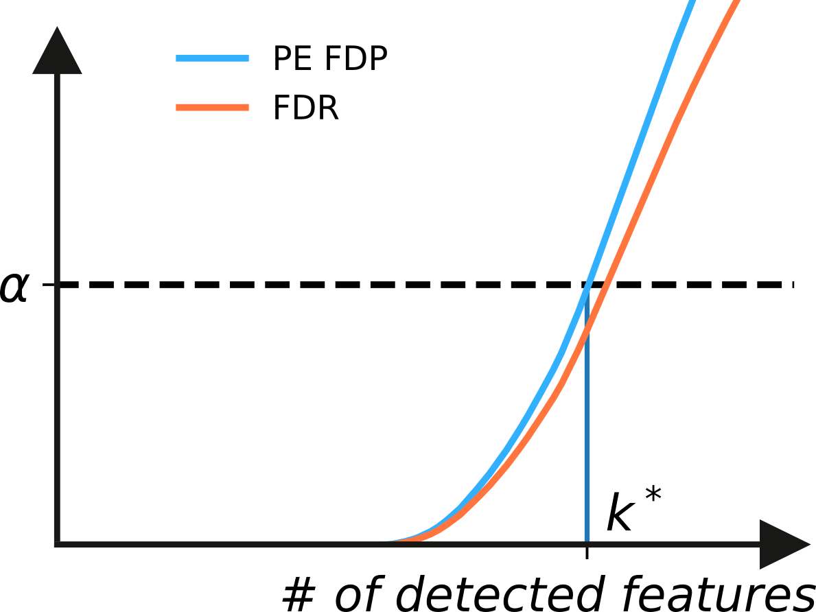
The obtained gene sets may be difficult to interpret for some users. For this reason, we provide a data-supported way to select \(\epsilon\), such that the posterior expected False Discovery Proportion (FDP) is below a significance level \(\alpha\). To clarify how to compute the posterior expectation, we introduce two notations. We denote

\begin{align} \mu^k_f = \begin{cases} 1 ~~\textrm{if feature $g$ is tagged DE} \\ 0 ~~\textrm{otherwise} \end{cases}, \end{align}

the decision rule tagging \(k\) features of highest \(p_f\) as DE. We also note \(d^f\) the binary random variable taking value 1 if feature \(f\) is differentially expressed.

The False Discovery Proportion is a random variable corresponding to the ratio of the number of false positives over the total number of predicted positives. For the specific family of decision rules \(\mu^k, k\) that we consider here, the FDP can be written as

\begin{align} FDP_{\mu^k} = \frac {\sum_f (1 - d^f) \mu_f^k} {\sum_f \mu_f^k} . \end{align}

However, note that the posterior expectation of \(d^f\), denoted as \(\mathbb{E}_{post}[.]\), verifies \(\mathbb{E}_{post}[FDP_{d^f}] = p^f\). Hence, by linearity of the expectation, we can estimate the false discovery rate corresponding to \(k\) detected features as

\[ \mathbb{E}_{post}[FDP_{\mu^k}] = \frac{\sum_f (1 - p^f) \mu_f^k}{\sum_f \mu_f^k}. \]

Hence, for a given significance level \(\alpha\), we select the maximum detections \(k^*\), such that \(\mathbb{E}_{post}[FDP_{\mu^k}] \leq \alpha\), as illustrated below.