scANVI#

scANVI [1] (single-cell ANnotation using Variational Inference; Python class SCANVI) is a semi-supervised model for single-cell transcriptomics data. In a sense, it can be seen as a scVI extension that can leverage the cell type knowledge for a subset of the cells present in the data sets to infer the states of the rest of the cells. For this reason, scANVI can help annotate a data set of unlabelled cells from manually annotated atlases, e.g., Tabula Sapiens [2].

The advantages of scANVI are:

Comprehensive in capabilities.
Scalable to very large datasets (>1 million cells).

The limitations of scANVI include:

Effectively requires a GPU for fast inference.
Latent space is not interpretable, unlike that of a linear method.
May not scale to very large number of cell types.

Preliminaries#

scANVI takes as input a scRNA-seq gene expression matrix \(X\) with \(N\) cells and \(G\) genes, as well as a vector \(\mathbf{c}\) containing the partially observed cell type annotations. Let \(C\) be the number of observed cell types in the data. Additionally, a design matrix \(S\) containing \(p\) observed covariates, such as day, donor, etc, is an optional input. While \(S\) can include both categorical covariates and continuous covariates, in the following, we assume it contains only one categorical covariate with \(K\) categories, which represents the common case of having multiple batches of data.

Generative process#

scANVI extends the scVI model by making use of observed cell types \(c_n\) following a graphical model inspired by works on semi-supervised VAEs [3].

\begin{align} c_n &\sim \mathrm{Categorical}(1/C, ..., 1/C) \\ u_n &\sim \mathcal{N}(0, I) \\ z_n &\sim \mathcal{N}(f_z^\mu(c_n, u_n), f_z^\sigma(c_n, u_n) \odot I) \\ \ell_n &\sim \mathrm{LogNormal}\left( \ell_\mu^\top s_n ,\ell_{\sigma^2}^\top s_n \right) \\ \rho _n &= f_w\left( z_n, s_n \right) \\ \pi_{ng} &= f_h^g(z_n, s_n) \\ x_{ng} &\sim \mathrm{ObservationModel}(\ell_n \rho_n, \theta_g, \pi_{ng}) \end{align}

We assume no knowledge over the distribution of cell types in the data (i.e., uniform probabilities for categorical distribution on \(c_n\)). This modeling choice helps ensure a proper handling of rare cell types in the data. We assume that the within-cell-type characterization of the cell follows a Normal distribution, s.t. \(u_n \sim \mathcal{N}(0, I_d)\). The distribution over the random vector \(z_n\) contains learnable parameters in the form of the neural networks \(f_z^\mu\), \(f_z^\sigma\). Qualitatively, \(z_n\) characterizes each cell cellular state as a continuous, low-dimensional random variable, and has the same interpretation as in the scVI model. However, the prior for this variable takes into account the partial cell-type information to better structure the latent space.

The rest of the model closely follows scVI. In particular, it represents the library size as a random variable, and gene expression likelihoods as negative binomial distributions parameterized by functions of \(z_n, \ell_n\), condition to the batch assignments \(s_n\).

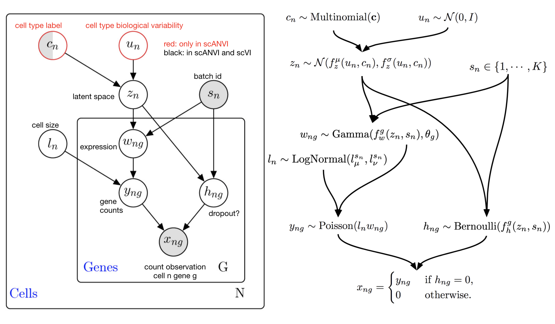
scANVI graphical model for the ZINB likelihood model. Note that this graphical model contains more latent variables than the presentation above. Marginalization of these latent variables leads to the ZINB observation model (math shown in publication supplement).#

In addition to the table in scVI, we have the following in scANVI.

Latent variable	Description	Code variable (if different)
\(c_n \in \Delta^{C-1}\)	Cell type.	`y`
\(z_n \in \mathbb{R}^{d}\)	Latent cell state	`z_1`
\(u_n \in \mathbb{R}^{d}\)	Latent cell-type specific state	`z_2`

Inference#

scANVI assumes the following factorization for the inference model

\begin{align} q_\eta(z_n, \ell_n, u_n, c_n \mid x_n) = q_\eta(z_n \mid x_n) q_\eta(\ell_n \mid x_n) q_\eta(c_n \mid z_n) q_\eta(u_n \mid c_n, z_n) \end{align}

We make several observations here. First, each of those variational distributions will be parameterized by neural networks. Second, while \(q_\eta(z_n, x_n)\) and \(q_\eta(u_n \mid c_n, z_n)\) are assumed Gaussian, \(q_\eta(c_n \mid z_n)\) corresponds to a Categorical distribution over cell types. In particular, the variational distribution \(q_\eta(c_n \mid z_n)\) can predict cell types for any cell.

Behind the scenes, scANVI’s classifier uses the mean of a cell’s variational distribution \(q_\eta(z_n \mid x_n)\) for classification.

Training details#

scANVI optimizes evidence lower bounds (ELBO) on the log evidence. For the sake of clarity, we ignore the library size and batch assignments below. We note that the evidence and hence the ELBO have a different expression for cells with observed and unobserved cell types.

First, assume that we observe both gene expressions \(x_n\) and type assignments \(c_n\). In that case, we bound the log evidence as

\begin{align} \log p_\theta(x_n, c_n) \geq \mathbb{E}_{q_\eta(z_n \mid x_n) q_\eta(u_n \mid z_n, c_n)} \left[ \log \frac { p_\theta(x_n, c_n, z_n, u_n) } { q_\eta(z_n \mid x_n) q_\eta(u_n \mid z_n, c_n) } \right] =: \mathcal{L}_S \end{align}

We aim to optimize for \(\theta, \eta\) the right-hand side of this equation using stochastic gradient descent. Gradient updates for the generative model parameters \(\theta\) are easy to get. In that case, the gradient of the expectation corresponds to the expectation of the gradients.

However, this is not the case when we differentiate for \(\eta\). The reparameterization trick solves this issue and applies to the (Gaussian) distributions associated with \(q_\eta(z_n \mid x_n) ,q_\eta(u_n \mid z_n, c_n)\). In particular, we can write \(\mathcal{L}_S\) as an expectation under noise distributions independent of \(\eta\). For convenience, we will write expectations of the form \(\mathbb{E}_{\epsilon_v}\) to denote expectation under the variational distribution using the reparameterization trick. We refer the reader to [4] for additional insight on the reparameterization trick.

\begin{align} \nabla_\eta \mathcal{L}_S := \mathbb{E}_{\epsilon_z, \epsilon_u} \left[ \nabla_\eta \log \frac { p_\theta(x_n, c_n, z_n, u_n) } { q_\eta(z_n \mid x_n) q_\eta(u_n \mid z_n, c_n) } \right] =: \mathcal{L}_S \end{align}

Things get trickier in the unobserved cell type case. In this setup, the ELBO corresponds to the right-hand side of

\begin{align} p_\theta(x_n) \geq \mathbb{E}_{ q_\eta(z_n \mid x_n) q_\eta(c_n \mid z_n) q_\eta(u_n \mid z_n, c_n) } \left[ \log \frac { p_\theta(x_n, c_n, z_n, u_n) } { q_\eta(z_n \mid x_n) q_\eta(c_n \mid z_n) q_\eta(u_n \mid z_n, c_n) } \right]=:\mathcal{L}_u \end{align}

Unfortunately, the reparameterization trick does not apply naturally to \(q_\eta(c_n \mid z_n)\). As an alternative, we observe that

\begin{align} \mathcal{L}_u = \mathbb{E}_{ \epsilon_z } \left[ \sum_{c=1}^C q_\eta(c_n=c \mid z_n) \mathbb{E}_{\epsilon_u} \left[ \log \frac { p_\theta(x_n, c_n=c, z_n, u_n) } { q_\eta(z_n \mid x_n) q_\eta(c_n \mid z_n) q_\eta(u_n \mid z_n, c_n=c) } \right] \right] \end{align}

In this form, we can differentiate \(\mathcal{L}_u\) with respect to the inference network parameters, as

\begin{align} \nabla_\eta \mathcal{L}_u = \mathbb{E}_{ \epsilon_z } \left[ \sum_{c=1}^C \nabla_\eta \left( q_\eta(c_n=c \mid z_n) \mathbb{E}_{\epsilon_u} \left[ \log \frac { p_\theta(x_n, c_n=c, z_n, u_n) } { q_\eta(z_n \mid x_n) q_\eta(c_n \mid z_n) q_\eta(u_n \mid z_n, c_n=c) } \right) \right] \right] \end{align}

In other words, we will need to marginalize \(c_n\) out to circumvent the fact that categorical distributions cannot use the reparameterization trick.

Overall, we optimize \(\mathcal{L} = \mathcal{L}_U + \mathcal{L}_S\) to train the model on both labeled and unlabelled data.

Tasks#

scANVI can perform all the same tasks as scVI (see scVI). In addition, scANVI can do the following:

Prediction#

For prediction, scANVI returns \(q_\eta(c_n \mid z_n)\) in the following function:

>>> adata.obs["scanvi_prediction"] = model.predict()