scVI

scVI [1] (single-cell Variational Inference; Python class SCVI) posits a flexible generative model of scRNA-seq count data that can subsequently be used for many common downstream tasks.

The advantages of scVI are:

• Comprehensive in capabilities.

• Scalable to very large datasets (>1 million cells).

The limitations of scVI include:

• Effectively requires a GPU for fast inference.

• Latent space is not interpretable, unlike that of a linear method.

Tutorials:

• Introduction to scvi-tools

• Atlas-level integration of lung data

• Reference mapping with scvi-tools

• Integrating datasets with scVI in R

Preliminaries

scVI takes as input a scRNA-seq gene expression matrix \(X\) with \(N\) cells and \(G\) genes. Additionally, a design matrix \(S\) containing \(p\) observed covariates, such as day, donor, etc, is an optional input. While \(S\) can include both categorical covariates and continuous covariates, in the following, we assume it contains only one categorical covariate with \(K\) categories, which represents the common case of having multiple batches of data.

Generative process

scVI posits that the observed UMI counts for cell \(n\) and gene \(g\), \(x_{ng}\), are generated by the following process:

\begin{align} z_n &\sim {\mathrm{Normal}}\left( {0,I} \right) \\ \ell_n &\sim \mathrm{LogNormal}\left( \ell_\mu^\top s_n ,\ell_{\sigma^2}^\top s_n \right) \\ \rho _n &= f_w\left( z_n, s_n \right) \\ \pi_{ng} &= f_h^g(z_n, s_n) \\ x_{ng} &\sim \mathrm{ObservationModel}(\ell_n \rho_n, \theta_g, \pi_{ng}) \end{align}

Succintly, the gene expression for each gene depends on a latent variable \(z_n\) that is cell-specific. The prior parameters \(\ell_\mu\) and \(\ell_{\sigma^2}\) are computed per batch as the mean and variance of the log library size over cells. The expression data are generated from a count-based likelihood distribution, which here, we denote as the \(\mathrm{ObservationModel}\). While by default the \(\mathrm{ObservationModel}\) is a \(\mathrm{ZeroInflatedNegativeBinomial}\) (ZINB) distribution parameterized by its mean, inverse dispersion, and non-zero-inflation probability, respectively, users can pass gene_likelihood = "negative_binomial" to SCVI, for example, to use a simpler \(\mathrm{NegativeBinomial}\) distribution.

The generative process of scVI uses two neural networks:

\begin{align} f_w(z_n, s_n) &: \mathbb{R}^{d} \times \{0, 1\}^K \to \Delta^{G-1}\\ f_h(z_n, s_n) &: \mathbb{R}^d \times \{0, 1\}^K \to (0, 1)^T \end{align}

which respectively decode the denoised gene expression and non-zero-inflation probability (only if using ZINB).

This generative process is also summarized in the following graphical model:

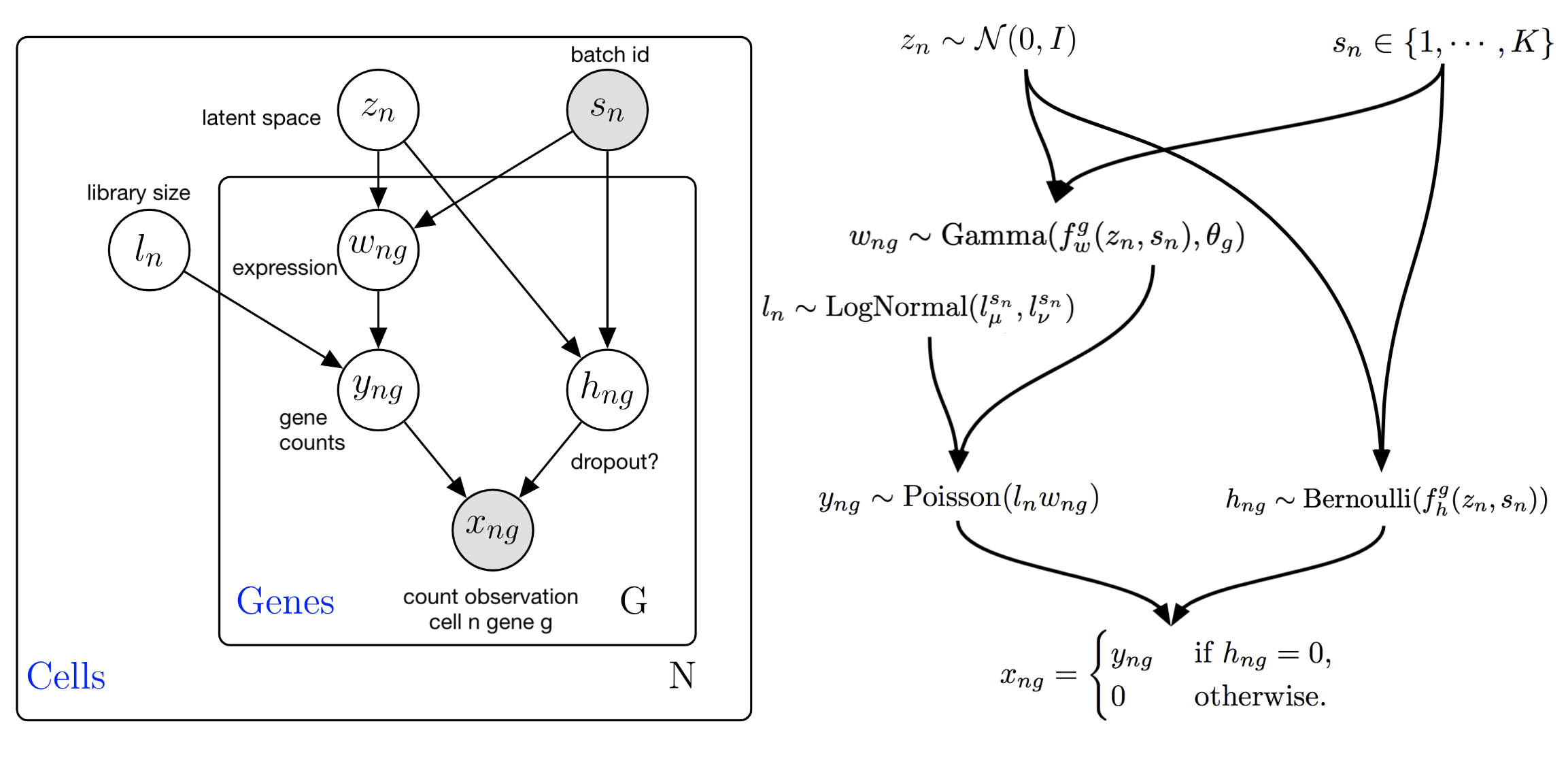
scVI graphical model for the ZINB likelihood model. Note that this graphical model contains more latent variables than the presentation above. Marginalization of these latent variables leads to the ZINB observation model (math shown in publication supplement).

The latent variables, along with their description are summarized in the following table:

Latent variable	Description	Code variable (if different)
\(z_n \in \mathbb{R}^d\)	Low-dimensional representation capturing the state of a cell.	N/A
\(\rho_n \in \Delta^{G-1}\)	Denoised/normalized gene expression. This is a vector that sums to 1 within a cell, unless size_factor_key is not None in setup_anndata, in which case this is only forced to be non-negative via softplus.	px_scale
\(\ell_n \in (0, \infty)\)	Library size for RNA. Here it is modeled as a latent variable, but the recent default for scVI is to treat library size as observed, equal to the total RNA UMI count of a cell. This can be controlled by passing use_observed_lib_size=False to SCVI. The library size can also be set manually using size_factor_key in setup_anndata.	N/A
\(\theta_g \in (0, \infty)\)	Inverse dispersion for negative binomial. This can be set to be gene/batch specific for example (and would thus be \(\theta_{kg}\)), by passing dispersion="gene-batch" during model intialization. Note that px_r also refers to the underlying real-valued torch parameter that is then exponentiated on every forward pass of the model.	px_r

Inference

scVI uses variational inference and specifically auto-encoding variational bayes (see Variational Inference) to learn both the model parameters (the neural network params, dispersion params, etc.) and an approximate posterior distribution with the following factorization:

\begin{align} q_\eta(z_n, \ell_n \mid x_n) := q_\eta(z_n \mid x_n, s_n)q_\eta(\ell_n \mid x_n). \end{align}

Here \(\eta\) is a set of parameters corresponding to inference neural networks (encoders), which we do not describe in detail here, but are described in the scVI paper. The underlying class used as the encoder for scVI is Encoder. In the case of use_observed_lib_size=True, \(q_\eta(\ell_n \mid x_n)\) can be written as a point mass on the observed library size.

It it important to note that by default, scVI only receives the expression data as input (i.e., not the observed cell-level covariates). Empirically, we have not seen much of a difference by having the encoder take as input the concatenation of these items (i.e., \(q_\eta(z_n, \ell_n \mid x_n, s_n)\), but users can control it manually by passing encode_covariates=True to scvi.model.SCVI.

Tasks

Here we provide an overview of some of the tasks that scVI can perform. Please see scvi.model.SCVI for the full API reference.

Dimensionality reduction

For dimensionality reduction, the mean of the approximate posterior \(q_\eta(z_n \mid x_n, s_n)\) is returned by default. This is achieved using the method:

>>> latent = model.get_latent_representation()
>>> adata.obsm["X_scvi"] = latent

Users may also return samples from this distribution, as opposed to the mean by passing the argument give_mean=False. The latent representation can be used to create a nearest neighbor graph with scanpy with:

>>> import scanpy as sc
>>> sc.pp.neighbors(adata, use_rep="X_scvi")
>>> adata.obsp["distances"]

Transfer learning

A scVI model can be pre-trained on reference data and updated with query data using load_query_data(), which then facilitates transfer of metadata like cell type annotations. See the Transfer learning guide for more information.

Normalization/denoising/imputation of expression

In get_normalized_expression() scVI returns the expected value of \(\rho_n\) under the approximate posterior. For one cell \(n\), this can be written as:

\begin{align} \mathbb{E}_{q_\eta(z_n \mid x_n)}\left[\ell_n'f_w\left( z_n, s_n \right) \right], \end{align}

where \(\ell_n'\) is by default set to 1. See the library_size parameter for more details. The expectation is approximated using Monte Carlo, and the number of samples can be passed as an argument in the code:

>>> model.get_normalized_expression(n_samples=10)

By default the mean over these samples is returned, but users may pass return_mean=False to retrieve all the samples.

Notably, this function also has the transform_batch parameter that allows counterfactual prediction of expression in an unobserved batch. See the Counterfactual prediction guide.

Differential expression

Differential expression analysis is achieved with differential_expression(). scVI tests differences in magnitude of \(f_w\left( z_n, s_n \right)\). More info is in Differential Expression.

Data simulation

Data can be generated from the model using the posterior predictive distribution in posterior_predictive_sample(). This is equivalent to feeding a cell through the model, sampling from the posterior distributions of the latent variables, retrieving the likelihood parameters (of \(p(x \mid z, s)\)), and finally, sampling from this distribution.

---

[1]

Romain Lopez, Jeffrey Regier, Michael Cole, Michael I. Jordan, Nir Yosef (2018), Deep generative modeling for single-cell transcriptomics, Nature Methods.