Using SHAP values and IntegratedGradients for cell type classification interpretability

Previously we saw semi-supervised models, like SCANVI being used for tasks like cell type classification, enabling researchers to uncover complex biological patterns. However, as these models become more sophisticated, it is essential to understand not just the predictions they make, but why they make them. This is where interpretability methods like SHAP (SHapley Additive exPlanations) and CAPTUM IntegratedGradients come into play. By providing insights into the influence of individual features on model predictions, these methods help us trust and validate our models in critical biological contexts.

In this tutorial, we’ll explore the significance of interpretability techniques in supervised cell classification using ScanVI, which are now avialble as part of SCVI-Tools.

Note

Running the following cell will install tutorial dependencies on Google Colab only. It will have no effect on environments other than Google Colab.

!pip install --quiet scvi-colab
from scvi_colab import install

install()

import matplotlib.pyplot as plt
import numpy as np
import pandas as pd
import scanpy as sc
import scvi
import seaborn as sns
import torch

torch.set_float32_matmul_precision("high")

scvi.settings.seed = 0
print("Last run with scvi-tools version:", scvi.__version__)

Last run with scvi-tools version: 1.4.2

Load data and train scanvi

In this tutorial we will be using the dataset of peripheral blood mononuclear cells from 10x Genomics, PBMC dataset

adata = scvi.data.pbmc_dataset()
adata.layers["counts"] = adata.X.copy()
adata.obs["batch"] = adata.obs["batch"].astype("category")
adata

INFO     File data/gene_info_pbmc.csv already downloaded                                                           
INFO     File data/pbmc_metadata.pickle already downloaded                                                         
INFO     File data/pbmc8k/filtered_gene_bc_matrices.tar.gz already downloaded                                      
INFO     Extracting tar file                                                                                       
INFO     Removing extracted data at data/pbmc8k/filtered_gene_bc_matrices                                          
INFO     File data/pbmc4k/filtered_gene_bc_matrices.tar.gz already downloaded                                      
INFO     Extracting tar file                                                                                       
INFO     Removing extracted data at data/pbmc4k/filtered_gene_bc_matrices

AnnData object with n_obs × n_vars = 11990 × 3346
    obs: 'n_counts', 'batch', 'labels', 'str_labels'
    var: 'gene_symbols', 'n_counts-0', 'n_counts-1', 'n_counts'
    uns: 'cell_types'
    obsm: 'design', 'raw_qc', 'normalized_qc', 'qc_pc'
    layers: 'counts'

adata.var_names = adata.var["gene_symbols"]

adata.obs.str_labels.value_counts()  # list of classes and their observations

str_labels
CD4 T cells          4996
CD14+ Monocytes      2227
B cells              1621
CD8 T cells          1448
Other                 463
NK cells              457
FCGR3A+ Monocytes     351
Dendritic Cells       339
Megakaryocytes         88
Name: count, dtype: int64

print("# cells, # genes before filtering:", adata.shape)

sc.pp.filter_genes(adata, min_counts=3)
sc.pp.filter_cells(adata, min_counts=3)

# cells, # genes before filtering: (11990, 3346)

# We select a small number of genes here, so our later interpretability analysis will be fast
sc.pp.highly_variable_genes(
    adata,
    n_top_genes=200,
    subset=True,
    layer="counts",
    flavor="seurat_v3",
    batch_key="batch",
)
print("# cells, # genes after filtering:", adata.shape)

# cells, # genes after filtering: (11990, 200)

scvi.model.SCANVI.setup_anndata(
    adata,
    layer="counts",
    batch_key="batch",
    labels_key="str_labels",
    unlabeled_category="unknown",
)

model = scvi.model.SCANVI(adata)
model

ScanVI Model with the following params: 
unlabeled_category: unknown, n_hidden: 128, n_latent: 10, n_layers: 1, dropout_rate: 0.1, dispersion: gene, 
gene_likelihood: zinb
Training status: Not Trained
Model's adata is minified?: False

model.train(
    max_epochs=100,
    early_stopping=True,
    check_val_every_n_epoch=1,
    train_size=0.8,
    validation_size=0.2,
    # accelerator="gpu",
    # devices=-1,
    # strategy="ddp_notebook_find_unused_parameters_true",
)

INFO     Training for 100 epochs.

Inspect scanvi training and test performance

adata.obsm["X_scANVI"] = model.get_latent_representation()

# use scVI latent space for UMAP generation
sc.pp.neighbors(adata, use_rep="X_scANVI", n_neighbors=30)

sc.tl.umap(adata, min_dist=0.3)

sc.pl.umap(adata, color=["str_labels", "batch"], ncols=2, wspace=0.4)

Next we will apply the 2 techniques for features interpretability and compare between them

Integrated Gradients

Integrated Gradients is a robust interpretability technique that attributes the output of a model to its input features by calculating the cumulative sum of gradients along a path from a baseline (typically zero or a neutral input) to the actual input. This approach provides a way to measure how each feature contributes to the model’s output in a smooth and consistent manner.

It is availble for any semi supervised model in SCVI-Tools by passing the ig_interpretability=True flag to the predict function.

predictions, attributions = model.predict(ig_interpretability=True)

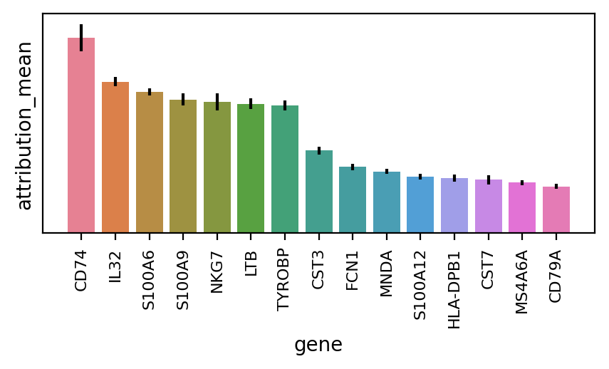
The method works relatievely fast and we can then plot the gene table with their importnace mean and variance, overall for all cell - types

n_plot = 15
attributions.head(n_plot)

	gene	gene_idx	attribution_mean	attribution_std	cells
0	CD74	70	1.046176	4.104647	11990
1	IL32	148	0.810820	1.358012	11990
2	S100A6	17	0.756088	1.103666	11990
3	S100A9	15	0.716369	1.809122	11990
4	NKG7	186	0.702932	2.459903	11990
5	LTB	78	0.692312	1.575437	11990
6	TYROBP	179	0.683626	1.525760	11990
7	CST3	166	0.441730	1.180127	11990
8	FCN1	104	0.354472	0.991154	11990
9	MNDA	20	0.329743	0.744831	11990
10	S100A12	16	0.302508	0.769542	11990
11	HLA-DPB1	81	0.296287	1.080156	11990
12	CST7	167	0.285223	1.292438	11990
13	MS4A6A	110	0.271008	0.730065	11990
14	CD79A	180	0.250256	0.732563	11990

df = attributions.head(n_plot)
ci = 1.96 * df["attribution_std"] / np.sqrt(df["cells"])
fig, ax = plt.subplots(nrows=1, ncols=1, figsize=(5, 2), dpi=200)
sns.barplot(ax=ax, data=df, x="gene", y="attribution_mean", hue="gene", dodge=False)
ax.set_yticks([])
plt.tick_params(axis="x", which="major", labelsize=8, labelrotation=90)
ax.errorbar(
    df["gene"].values,
    df["attribution_mean"].values,
    yerr=ci,
    ecolor="black",
    fmt="none",
)
if ax.get_legend() is not None:
    ax.get_legend().remove()

We can repeat for specific class (‘Dendritic Cells’):

predictions_class, attributions_class = model.predict(
    indices=np.where(adata.obs.str_labels == "Dendritic Cells")[0].tolist(),
    ig_interpretability=True,
)

attributions_class.head(n_plot)

	gene	gene_idx	attribution_mean	attribution_std	cells
0	CD74	70	5.473364	0.948142	339
1	FCER1A	21	3.630613	1.943166	339
2	HLA-DPB1	81	3.318439	0.631406	339
3	VIM	117	1.793772	0.506637	339
4	ANXA1	97	1.650854	0.695445	339
5	HLA-DMB	79	1.374406	0.584015	339
6	CLEC10A	157	1.342435	1.255666	339
7	HLA-DMA	80	1.158052	0.371506	339
8	COTL1	154	1.053837	0.387444	339
9	TYROBP	179	0.987148	0.421023	339
10	S100A10	13	0.952728	0.462643	339
11	ALDH2	130	0.767798	0.441154	339
12	PHACTR1	75	0.702436	0.534552	339
13	CAPG	31	0.656638	0.390209	339
14	LGALS3	141	0.514238	0.382886	339

df_class = attributions_class.head(n_plot)
ci = 1.96 * df_class["attribution_std"] / np.sqrt(df_class["cells"])
fig, ax = plt.subplots(nrows=1, ncols=1, figsize=(5, 2), dpi=200)
sns.barplot(ax=ax, data=df_class, x="gene", y="attribution_mean", hue="gene", dodge=False)
ax.set_yticks([])
plt.tick_params(axis="x", which="major", labelsize=8, labelrotation=90)
ax.errorbar(
    df_class["gene"].values,
    df_class["attribution_mean"].values,
    yerr=ci,
    ecolor="black",
    fmt="none",
)
if ax.get_legend() is not None:
    ax.get_legend().remove()

As expected, for a specific class, we can see different important genes, altough S100A4 is still the top contributer

More generally we would like to see a more general view of top genes to contribute to our celltype groups classification.

classes = adata.obs.str_labels.cat.categories
features = adata.var_names
attributions_class_pos_agg = pd.DataFrame()
n_cols = 3
top_n = 5
nrows = round(classes.size / n_cols)
fig, ax = plt.subplots(nrows, n_cols, sharex=False, figsize=(20, 20))
for idx, ct in enumerate(classes):
    _, attributions_class = model.predict(
        indices=np.where(adata.obs.str_labels == ct)[0].tolist(),
        ig_interpretability=True,
    )
    positive = attributions_class.head(top_n)
    positive["contribution"] = "positive"
    negative = attributions_class.tail(top_n)
    negative["contribution"] = "negative"
    avg = pd.concat([positive, negative])
    title = f"IG importance for: {ct}"

    # also keep the positive contributions
    attributions_class_pos = attributions_class[attributions_class.attribution_mean > 0]
    attributions_class_pos["class"] = ct
    attributions_class_pos_agg = pd.concat([attributions_class_pos_agg, attributions_class_pos])

    sns.barplot(
        x="attribution_mean",
        y="gene",
        hue="contribution",
        palette=["blue", "red"],
        data=avg,
        ax=ax[idx // n_cols, idx % n_cols],
    )

    ax[idx // n_cols, idx % n_cols].set_title(title)
    ax[idx // n_cols, idx % n_cols].legend(title="IG Contribution", loc="lower right")

_ = [fig.delaxes(ax_) for ax_ in ax.flatten() if not ax_.has_data()]

fig.tight_layout()

And we can also show the positive contribution of each gene being aggregated per cell type group

top_n = 20
# Pivot the data so that each group becomes a column for stacking
pivot_df = attributions_class_pos_agg.pivot_table(
    index="gene", columns="class", values="attribution_mean", aggfunc="sum"
)

# Sort by the total sum of each feature (sum across all groups)
pivot_df["total"] = pivot_df.sum(axis=1)  # Calculate the total sum for each feature
pivot_df = pivot_df.sort_values(by="total", ascending=False)  # Sort by the total value
pivot_df = pivot_df.head(top_n)  # Select the top 10 features

# Plotting the horizontal stacked bar plot
ax = pivot_df.drop("total", axis=1).plot(
    kind="barh", stacked=True, figsize=(10, 6), colormap="tab20"
)

# Add labels and title
ax.set_xlabel("IG Contribution Value")
ax.set_ylabel("Gene")
ax.set_title("Top 10 Stacked IG Contributions by Cell Type per Gene")

# Display the plot
plt.tight_layout()
plt.show()

SHAP

SHAP (SHapley Additive exPlanations) values are a popular interpretability technique based on cooperative game theory. The core idea is to fairly allocate the “credit” for a model’s prediction to each feature, by considering all possible combinations of features and their impact on the prediction. SHAP values are additive, meaning the sum of the SHAP values for all features equals the difference between the model’s output and the average prediction. This method works for any model type, providing a consistent way to explain individual predictions, making it highly versatile and widely applicable. Deep SHAP is an extension of the SHAP method designed specifically for deep learning models, such as the ones in SCVI-Tools. For more information see this

Calcualtion of SHAP for SC data usually takes a lot of time. In SCVI-Tools we are running an approximation of FastSHAP in order to reduce runtime, where we train a shallow surrogate model to imitate the original model prediction and than run the SHAP over the surrogate model. See this

import torch.nn as nn
from scvi.utils import FastSHAP, Surrogate
from scvi.utils.fastshap import KLDivLoss, MaskLayer1d

num_features = len(features)
num_classes = len(classes)
surr = nn.Sequential(
    MaskLayer1d(value=0, append=True),
    nn.Linear(2 * num_features, 128),
    nn.ELU(inplace=True),
    nn.Linear(128, 128),
    nn.ELU(inplace=True),
    nn.Linear(128, num_classes),
).to(model.device)

# Set up surrogate object
surrogate = Surrogate(surr, num_features)
# Train Surrogate
surrogate.train_original_model(
    train_data=adata.X.toarray()[model.train_indices],
    val_data=adata.X.toarray()[model.validation_indices],
    original_model=model.shap_adata_predict,
    batch_size=64,
    max_epochs=10,
    loss_fn=KLDivLoss(),
    validation_samples=10,
    validation_batch_size=10000,
    verbose=True,
)

# Train FastSHAP
# Create explainer model
explainer = nn.Sequential(
    nn.Linear(num_features, 128),
    nn.ReLU(inplace=True),
    nn.Linear(128, 128),
    nn.ReLU(inplace=True),
    nn.Linear(128, num_classes * num_features),
).to(model.device)

# Set up FastSHAP object
fastshap = FastSHAP(explainer, surrogate, normalization="additive", link=nn.Softmax(dim=-1))
# Train
fastshap.train(
    train_data=adata.X.toarray()[model.train_indices],
    val_data=adata.X.toarray()[model.validation_indices],
    batch_size=32,
    num_samples=32,
    max_epochs=100,
    validation_samples=128,
    verbose=True,
)

----- Epoch = 1 -----
Val loss = 5.208660

New best epoch, loss = 5.208660

----- Epoch = 2 -----
Val loss = 1.557097

New best epoch, loss = 1.557097

----- Epoch = 3 -----
Val loss = 0.361534

New best epoch, loss = 0.361534

----- Epoch = 4 -----
Val loss = 0.076193

New best epoch, loss = 0.076193

----- Epoch = 5 -----
Val loss = 0.025957

New best epoch, loss = 0.025957

----- Epoch = 6 -----
Val loss = 0.017574

New best epoch, loss = 0.017574

----- Epoch = 7 -----
Val loss = 0.015273

New best epoch, loss = 0.015273

----- Epoch = 8 -----
Val loss = 0.014053

New best epoch, loss = 0.014053

----- Epoch = 9 -----
Val loss = 0.013188

New best epoch, loss = 0.013188

----- Epoch = 10 -----
Val loss = 0.012649

New best epoch, loss = 0.012649

----- Epoch = 11 -----
Val loss = 0.012275

New best epoch, loss = 0.012275

----- Epoch = 12 -----
Val loss = 0.012005

New best epoch, loss = 0.012005

----- Epoch = 13 -----
Val loss = 0.011791

New best epoch, loss = 0.011791

----- Epoch = 14 -----
Val loss = 0.011636

New best epoch, loss = 0.011636

----- Epoch = 15 -----
Val loss = 0.011542

New best epoch, loss = 0.011542

----- Epoch = 16 -----
Val loss = 0.011452

New best epoch, loss = 0.011452

----- Epoch = 17 -----
Val loss = 0.011388

New best epoch, loss = 0.011388

----- Epoch = 18 -----
Val loss = 0.011344

New best epoch, loss = 0.011344

----- Epoch = 19 -----
Val loss = 0.011303

New best epoch, loss = 0.011303

----- Epoch = 20 -----
Val loss = 0.011292

New best epoch, loss = 0.011292

----- Epoch = 21 -----
Val loss = 0.011278

New best epoch, loss = 0.011278

----- Epoch = 22 -----
Val loss = 0.011252

New best epoch, loss = 0.011252

----- Epoch = 23 -----
Val loss = 0.011260

----- Epoch = 24 -----
Val loss = 0.011253

----- Epoch = 25 -----
Val loss = 0.011250

New best epoch, loss = 0.011250

----- Epoch = 26 -----
Val loss = 0.011243

New best epoch, loss = 0.011243

----- Epoch = 27 -----
Val loss = 0.011241

New best epoch, loss = 0.011241

----- Epoch = 28 -----
Val loss = 0.011233

New best epoch, loss = 0.011233

----- Epoch = 29 -----
Val loss = 0.011236

----- Epoch = 30 -----
Val loss = 0.011229

New best epoch, loss = 0.011229

----- Epoch = 31 -----
Val loss = 0.011229

New best epoch, loss = 0.011229

----- Epoch = 32 -----
Val loss = 0.011239

----- Epoch = 33 -----
Val loss = 0.011232

----- Epoch = 34 -----
Val loss = 0.011167

New best epoch, loss = 0.011167

----- Epoch = 35 -----
Val loss = 0.011160

New best epoch, loss = 0.011160

----- Epoch = 36 -----
Val loss = 0.011163

----- Epoch = 37 -----
Val loss = 0.011170

----- Epoch = 38 -----
Val loss = 0.011168

----- Epoch = 39 -----
Val loss = 0.011133

New best epoch, loss = 0.011133

----- Epoch = 40 -----
Val loss = 0.011129

New best epoch, loss = 0.011129

----- Epoch = 41 -----
Val loss = 0.011131

----- Epoch = 42 -----
Val loss = 0.011133

----- Epoch = 43 -----
Val loss = 0.011128

New best epoch, loss = 0.011128

----- Epoch = 44 -----
Val loss = 0.011136

----- Epoch = 45 -----
Val loss = 0.011136

----- Epoch = 46 -----
Val loss = 0.011137

----- Epoch = 47 -----
Val loss = 0.011119

New best epoch, loss = 0.011119

----- Epoch = 48 -----
Val loss = 0.011114

New best epoch, loss = 0.011114

----- Epoch = 49 -----
Val loss = 0.011113

New best epoch, loss = 0.011113

----- Epoch = 50 -----
Val loss = 0.011115

----- Epoch = 51 -----
Val loss = 0.011115

----- Epoch = 52 -----
Val loss = 0.011108

New best epoch, loss = 0.011108

----- Epoch = 53 -----
Val loss = 0.011101

New best epoch, loss = 0.011101

----- Epoch = 54 -----
Val loss = 0.011103

----- Epoch = 55 -----
Val loss = 0.011102

----- Epoch = 56 -----
Val loss = 0.011101

New best epoch, loss = 0.011101

----- Epoch = 57 -----
Val loss = 0.011100

New best epoch, loss = 0.011100

----- Epoch = 58 -----
Val loss = 0.011099

New best epoch, loss = 0.011099

----- Epoch = 59 -----
Val loss = 0.011098

New best epoch, loss = 0.011098

----- Epoch = 60 -----
Val loss = 0.011100

----- Epoch = 61 -----
Val loss = 0.011100

----- Epoch = 62 -----
Val loss = 0.011100

----- Epoch = 63 -----
Val loss = 0.011099

----- Epoch = 64 -----
Val loss = 0.011100

Stopping early at epoch = 63

We repeat the same figure plot like the previous case:

classes = adata.obs.str_labels.cat.categories
features = adata.var_names
attributions_class_pos_agg = pd.DataFrame()
n_cols = 3
top_n = 5
nrows = round(classes.size / n_cols)
fig, ax = plt.subplots(nrows, n_cols, sharex=False, figsize=(20, 20))
for idx, ct in enumerate(classes):
    sum_shap_per_class = [0] * num_features
    for ind in np.where(adata.obs.str_labels == ct)[0].tolist():
        sum_shap_per_class += fastshap.shap_values(np.array([adata.X[ind].toarray()]))[0][:, 0]
    attributions_class = pd.DataFrame(
        {"gene": features, "mean_shap": sum_shap_per_class / num_features, "class": ct}
    ).sort_values("mean_shap", ascending=False)

    positive = attributions_class.head(top_n)
    positive["contribution"] = "positive"
    negative = attributions_class.tail(top_n)
    negative["contribution"] = "negative"
    avg = pd.concat([positive, negative])
    title = f"IG importance for: {ct}"

    # also keep the positive contributions
    attributions_class_pos = attributions_class[attributions_class.mean_shap > 0]
    attributions_class_pos["class"] = ct
    attributions_class_pos_agg = pd.concat([attributions_class_pos_agg, attributions_class_pos])

    sns.barplot(
        x="mean_shap",
        y="gene",
        hue="contribution",
        palette=["blue", "red"],
        data=avg,
        ax=ax[idx // n_cols, idx % n_cols],
    )

    ax[idx // n_cols, idx % n_cols].set_title(title)
    ax[idx // n_cols, idx % n_cols].legend(title="SHAP Contribution", loc="lower right")

_ = [fig.delaxes(ax_) for ax_ in ax.flatten() if not ax_.has_data()]

fig.tight_layout()

top_n = 20
# Pivot the data so that each group becomes a column for stacking
pivot_df = attributions_class_pos_agg.pivot_table(
    index="gene", columns="class", values="mean_shap", aggfunc="sum"
)

# Sort by the total sum of each feature (sum across all groups)
pivot_df["total"] = pivot_df.sum(axis=1)  # Calculate the total sum for each feature
pivot_df = pivot_df.sort_values(by="total", ascending=False)  # Sort by the total value
pivot_df = pivot_df.head(top_n)  # Select the top 10 features

# Plotting the horizontal stacked bar plot
ax = pivot_df.drop("total", axis=1).plot(
    kind="barh", stacked=True, figsize=(10, 6), colormap="tab20"
)

# Add labels and title
ax.set_xlabel("SHAP Contribution Value")
ax.set_ylabel("Gene")
ax.set_title("Top 10 Stacked SHAP Contributions by Cell Type per Gene")

# Display the plot
plt.tight_layout()
plt.show()

And we can see some overlapping genes from the 2 methods for this specific group of cells

As for SCVI-tools v1.3 Work on SHAP is still in progress: please check back in the next release!