MrVI analysis over Tahoe100M cells dataset using LaminDB Custom Dataloader

MrVI (Multi-resolution Variational Inference) is a model for analyzing multi-sample single-cell RNA-seq data. This tutorial show how to do run MrVI in PyTorch version over the Tahoe100M cells dataset and perform basic analysis, using Lamin custom dataloader.

!pip install --quiet scvi-colab
from scvi_colab import install

install()

import gc
import tempfile

import matplotlib.pyplot as plt
import numpy as np
import pandas as pd
import scanpy as sc
import scvi
import scvi.hub
import seaborn as sns
import torch
from scvi.dataloaders import MappedCollectionDataModule
from scvi.external import MRVI

run_autotune = False

# import inspect
# print(inspect.getsource(MRVI))

# os.system("lamin init --storage ./lamindb_collection")
import lamindb as ln
# ln.setup.init()

→ connected lamindb: anonymous/lamindb_collection

scvi.settings.seed = 0
print("Last run with scvi-tools version:", scvi.__version__)

Last run with scvi-tools version: 1.3.3

sc.set_figure_params(figsize=(6, 6), frameon=False)
sns.set_theme()
torch.set_float32_matmul_precision("high")
save_dir = tempfile.TemporaryDirectory()

%config InlineBackend.print_figure_kwargs={"facecolor": "w"}
%config InlineBackend.figure_format="retina"

pd.set_option("display.max_rows", 50)
pd.set_option("display.max_columns", 50)
pd.set_option("display.width", 1000)

Get the data

We start by downloading the model from its hub in order to use its metadata Note that the model is very large therefore it will take time to being download.

# get the hub data
tahoe_hubmodel = scvi.hub.HubModel.pull_from_huggingface_hub(
    repo_name="vevotx/Tahoe-100M-SCVI-v1", cache_dir="."
)

tahoe_hubmodel.model.adata.obs.head()

INFO     Loading model...                                                                                          
INFO     File ./models--vevotx--Tahoe-100M-SCVI-v1/snapshots/b5283a73fbbed812a95264ace360da538b20af89/model.pt     
         already downloaded

	sample	species	gene_count	tscp_count	mread_count	bc1_wind	bc2_wind	bc3_wind	bc1_well	bc2_well	bc3_well	id	drugname_drugconc	drug	INT_ID	NUM.SNPS	NUM.READS	demuxlet_call	BEST.LLK	NEXT.LLK	DIFF.LLK.BEST.NEXT	BEST.POSTERIOR	SNG.POSTERIOR	SNG.BEST.LLK	SNG.NEXT.LLK	SNG.ONLY.POSTERIOR	DBL.BEST.LLK	DIFF.LLK.SNG.DBL	sublibrary	BARCODE	pcnt_mito	S_score	G2M_score	phase	pass_filter	dataset	_scvi_batch	_scvi_labels	_scvi_observed_lib_size	plate	Cell_Name_Vevo	Cell_ID_Cellosaur	observed_lib_size
BARCODE_SUB_LIB_ID
01_001_052-lib_1105	smp_1783	hg38	1878	2893	3284	1	1	52	A1	A1	E4	recgIHRi9MiCIr4CO	[('8-Hydroxyquinoline', 0.05, 'uM')]	8-Hydroxyquinoline	1.0	199.0	215.0	singlet	-50.74	-59.04	8.30	-55.0	1.0	-50.74	-87.96	0.0	-59.04	8.30	lib_1105	01_001_052	0.019357	0.174603	0.179670	G2M	full	0	0	0	2893	4	PANC-1	CVCL_0480	2893
01_001_105-lib_1105	smp_1783	hg38	1765	2434	2764	1	1	105	A1	A1	p2.A9	recgIHRi9MiCIr4CO	[('8-Hydroxyquinoline', 0.05, 'uM')]	8-Hydroxyquinoline	3.0	137.0	140.0	singlet	-37.97	-42.41	4.44	-43.0	1.0	-37.97	-64.52	0.0	-42.41	4.44	lib_1105	01_001_105	0.029581	0.297619	0.342857	G2M	full	0	0	0	2434	4	SW480	CVCL_0546	2434
01_001_165-lib_1105	smp_1783	hg38	3174	5691	6454	1	1	165	A1	A1	p2.F9	recgIHRi9MiCIr4CO	[('8-Hydroxyquinoline', 0.05, 'uM')]	8-Hydroxyquinoline	4.0	379.0	396.0	singlet	-129.66	-130.65	0.99	-130.0	1.0	-129.66	-186.89	0.0	-130.65	0.99	lib_1105	01_001_165	0.031629	0.031746	0.099084	G2M	full	0	0	0	5691	4	SW1417	CVCL_1717	5691
01_003_094-lib_1105	smp_1783	hg38	1380	1804	2050	1	3	94	A1	A3	H10	recgIHRi9MiCIr4CO	[('8-Hydroxyquinoline', 0.05, 'uM')]	8-Hydroxyquinoline	7.0	122.0	125.0	singlet	-31.79	-33.98	2.19	-36.0	1.0	-31.79	-49.36	0.0	-33.98	2.19	lib_1105	01_003_094	0.017738	-0.063492	0.019780	G2M	full	0	0	0	1804	4	SW1417	CVCL_1717	1804
01_003_164-lib_1105	smp_1783	hg38	1179	1514	1715	1	3	164	A1	A3	p2.F8	recgIHRi9MiCIr4CO	[('8-Hydroxyquinoline', 0.05, 'uM')]	8-Hydroxyquinoline	8.0	87.0	93.0	singlet	-28.99	-27.07	-1.92	-34.0	1.0	-28.99	-41.61	0.0	-27.07	-1.92	lib_1105	01_003_164	0.023118	-0.075397	-0.070879	G1	full	0	0	0	1514	4	A498	CVCL_1056	1514

# Load Cell Line Metadata
cell_lines = pd.read_csv(
    "/home/access/PycharmProjects/scvi-tools/Tahoe100M/cell_line_metadata.h5ad"
)
cell_lines.head()

	Unnamed: 0	cell_name	Cell_ID_DepMap	Cell_ID_Cellosaur	Organ	Driver_Gene_Symbol	Driver_VarZyg	Driver_VarType	Driver_ProtEffect_or_CdnaEffect	Driver_Mech_InferDM	Driver_GeneType_DM
0	0	A549	ACH-000681	CVCL_0023	Lung	CDKN2A	Hom	Deletion	DEL	LoF	Suppressor
1	1	A549	ACH-000681	CVCL_0023	Lung	CDKN2B	Hom	Deletion	DEL	LoF	Suppressor
2	2	A549	ACH-000681	CVCL_0023	Lung	KRAS	Hom	Missense	p.G12S	GoF	Oncogene
3	3	A549	ACH-000681	CVCL_0023	Lung	SMARCA4	Hom	Frameshift	p.Q729fs	LoF	Suppressor
4	4	A549	ACH-000681	CVCL_0023	Lung	STK11	Hom	Stopgain	p.Q37*	LoF	Suppressor

In the next part we are creating artifacts from a subset of 1M cells per plate (and 5 plates) from the dataset and unite them to a collection. Artifacts and collections are the ways lamindb interactes with the data. From this point forward we will not use adatas again. The tutorial assumed those files were already ready (see for how to here)

# Init Lamin instance
ln.track()

→ loaded Transform('GMYJf4FqDHnZ0000'), re-started Run('5FGprgCv...') at 2025-08-20 15:14:06 UTC
• recommendation: to identify the notebook across renames, pass the uid: ln.track("GMYJf4FqDHnZ")

# We make a collection of artifactos from files that are stored on disk
artifact1 = ln.Artifact.from_anndata(
    "/home/access/PycharmProjects/scvi-tools/Tahoe100M/tahoe100m_sample_1000000_plate1.h5ad",
    key="part_1.h5ad",
).save()
artifact2 = ln.Artifact.from_anndata(
    "/home/access/PycharmProjects/scvi-tools/Tahoe100M/tahoe100m_sample_1000000_plate2.h5ad",
    key="part_2.h5ad",
).save()
artifact3 = ln.Artifact.from_anndata(
    "/home/access/PycharmProjects/scvi-tools/Tahoe100M/tahoe100m_sample_1000000_plate3.h5ad",
    key="part_3.h5ad",
).save()
artifact4 = ln.Artifact.from_anndata(
    "/home/access/PycharmProjects/scvi-tools/Tahoe100M/tahoe100m_sample_1000000_plate4.h5ad",
    key="part_4.h5ad",
).save()
artifact5 = ln.Artifact.from_anndata(
    "/home/access/PycharmProjects/scvi-tools/Tahoe100M/tahoe100m_sample_1000000_rand.h5ad",
    key="part_5.h5ad",
).save()

! calling anonymously, will miss private instances
→ returning existing artifact with same hash: Artifact(uid='sBdR09Afz0MqbLu50002', is_latest=True, key='part_1.h5ad', suffix='.h5ad', kind='dataset', otype='AnnData', size=17933581240, hash='fmr6LyB4ySH0Q7vA_zCZMy', n_observations=1000000, branch_id=1, space_id=1, storage_id=1, run_id=2, created_by_id=1, created_at=2025-08-07 13:24:38 UTC); to track this artifact as an input, use: ln.Artifact.get()
→ returning existing artifact with same hash: Artifact(uid='6PuwYTVC0rc8ik9h0002', is_latest=True, key='part_2.h5ad', suffix='.h5ad', kind='dataset', otype='AnnData', size=19205241784, hash='Kd0DjdW_GFI2QXzeaFePJ2', n_observations=1000000, branch_id=1, space_id=1, storage_id=1, run_id=2, created_by_id=1, created_at=2025-08-07 13:24:49 UTC); to track this artifact as an input, use: ln.Artifact.get()
→ returning existing artifact with same hash: Artifact(uid='Y4Ht6CkaiGsXWWTJ0000', is_latest=True, key='part_3.h5ad', suffix='.h5ad', kind='dataset', otype='AnnData', size=15146243320, hash='f3_p_AkcSfh-P2aKlmOkeC', n_observations=1000000, branch_id=1, space_id=1, storage_id=1, run_id=2, created_by_id=1, created_at=2025-08-07 13:25:00 UTC); to track this artifact as an input, use: ln.Artifact.get()
→ returning existing artifact with same hash: Artifact(uid='GBKhWVRoRltw7UZk0001', is_latest=True, key='part_4.h5ad', suffix='.h5ad', kind='dataset', otype='AnnData', size=15207127144, hash='rJLJdKpkSvkvB-ks7A2z3e', n_observations=1000000, branch_id=1, space_id=1, storage_id=1, run_id=2, created_by_id=1, created_at=2025-08-07 13:25:11 UTC); to track this artifact as an input, use: ln.Artifact.get()
→ returning existing artifact with same hash: Artifact(uid='NBFiWx43U3hNm4dR0001', is_latest=True, key='part_5.h5ad', suffix='.h5ad', kind='dataset', otype='AnnData', size=17240836184, hash='7RX84cxLdX92Sb9Cu74ZjF', n_observations=1000000, branch_id=1, space_id=1, storage_id=1, run_id=2, created_by_id=1, created_at=2025-08-07 13:25:20 UTC); to track this artifact as an input, use: ln.Artifact.get()

collection = ln.Collection([artifact1, artifact2, artifact3, artifact4, artifact5], key="gather")
collection.save()

! returning existing collection with same hash: Collection(uid='6IASvDXmFbji3Uzu000Q', is_latest=True, key='gather', hash='5K17S6WOKo9udA6RiGW4Lw', branch_id=1, space_id=1, created_by_id=1, run_id=2, created_at=2025-08-07 13:25:33 UTC); if you intended to query to track this collection as an input, use: ln.Collection.get()

Collection(uid='6IASvDXmFbji3Uzu000Q', is_latest=True, key='gather', hash='5K17S6WOKo9udA6RiGW4Lw', branch_id=1, space_id=1, created_by_id=1, run_id=2, created_at=2025-08-07 13:25:33 UTC)

# We load the collection to see it consists of many h5ad files
artifacts = collection.artifacts.all()
artifacts.df()

	uid	key	description	suffix	kind	otype	size	hash	n_files	n_observations	_hash_type	_key_is_virtual	_overwrite_versions	space_id	storage_id	schema_id	version	is_latest	run_id	created_at	created_by_id	_aux	branch_id
id
39	sBdR09Afz0MqbLu50002	part_1.h5ad	None	.h5ad	dataset	AnnData	17933581240	fmr6LyB4ySH0Q7vA_zCZMy	None	1000000	sha1-fl	True	False	1	1	None	None	True	2	2025-08-07 13:24:38.913000+00:00	1	None	1
40	6PuwYTVC0rc8ik9h0002	part_2.h5ad	None	.h5ad	dataset	AnnData	19205241784	Kd0DjdW_GFI2QXzeaFePJ2	None	1000000	sha1-fl	True	False	1	1	None	None	True	2	2025-08-07 13:24:49.589000+00:00	1	None	1
41	Y4Ht6CkaiGsXWWTJ0000	part_3.h5ad	None	.h5ad	dataset	AnnData	15146243320	f3_p_AkcSfh-P2aKlmOkeC	None	1000000	sha1-fl	True	False	1	1	None	None	True	2	2025-08-07 13:25:00.960000+00:00	1	None	1
42	GBKhWVRoRltw7UZk0001	part_4.h5ad	None	.h5ad	dataset	AnnData	15207127144	rJLJdKpkSvkvB-ks7A2z3e	None	1000000	sha1-fl	True	False	1	1	None	None	True	2	2025-08-07 13:25:11.405000+00:00	1	None	1
43	NBFiWx43U3hNm4dR0001	part_5.h5ad	None	.h5ad	dataset	AnnData	17240836184	7RX84cxLdX92Sb9Cu74ZjF	None	1000000	sha1-fl	True	False	1	1	None	None	True	2	2025-08-07 13:25:20.940000+00:00	1	None	1

we can now define the batch and data loader which replaces the default AnnDataloder of and use that on MRVI model.

datamodule = MappedCollectionDataModule(
    collection,
    batch_key="plate",
    sample_key="sample",
    batch_size=1024,
    shuffle=True,
    join="inner",
    model_name="TorchMRVI",
    collection_val=collection,
)

print(datamodule.n_obs, datamodule.n_vars, datamodule.n_batch)

5000000 62710 14

Train mrVI with LaminDB

We will initialize the MRVI model with its “pytorch” backend. A JAX backend version can be also be used using backend=”jax”.

# Init the model
model = MRVI(registry=datamodule.registry, backend="torch")

# Training the model (for 5M cells will take 1 day+ with early stopping - better to cancel it)
import time

gc.collect()
start = time.time()
model.train(
    max_epochs=50,
    # early_stopping=True,
    plan_kwargs={"lr": 1e-3, "n_epochs_kl_warmup": 40},
    datamodule=datamodule,
    batch_size=1024,
    # early_stopping_patience=5,
    # check_val_every_n_epoch=1,
    # datasplitter_kwargs={
    #    "external_indexing": [np.array(train_ind), np.array(valid_ind)]
    # }
)
end = time.time()
print(f"Elapsed time: {end - start:.2f} seconds")

Elapsed time: 75375.09 seconds

model.history.keys()

dict_keys(['kl_weight', 'train_loss_step', 'validation_loss', 'elbo_validation', 'reconstruction_loss_validation', 'kl_local_validation', 'kl_global_validation', 'train_loss_epoch', 'elbo_train', 'reconstruction_loss_train', 'kl_local_train', 'kl_global_train'])

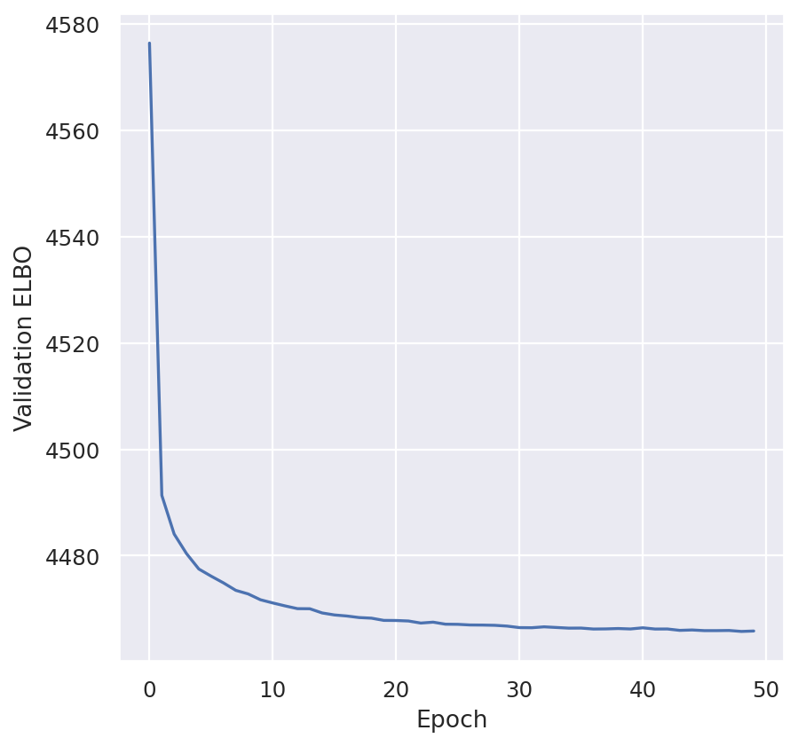
plt.plot(model.history["elbo_validation"])
plt.xlabel("Epoch")
plt.ylabel("Validation ELBO")
plt.show()

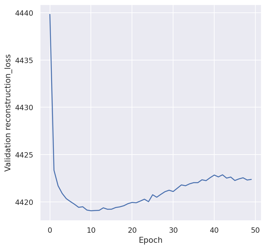
plt.plot(model.history["reconstruction_loss_validation"])
plt.xlabel("Epoch")
plt.ylabel("Validation reconstruction_loss")
plt.show()

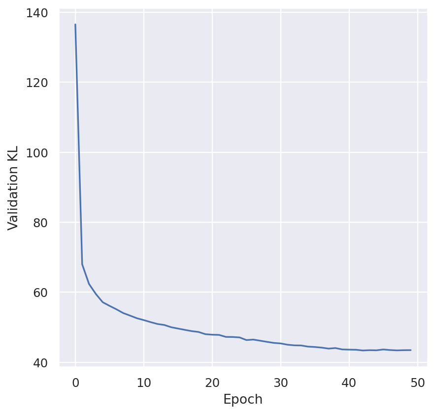
plt.plot(model.history["kl_local_validation"])
plt.xlabel("Epoch")
plt.ylabel("Validation KL")
plt.show()

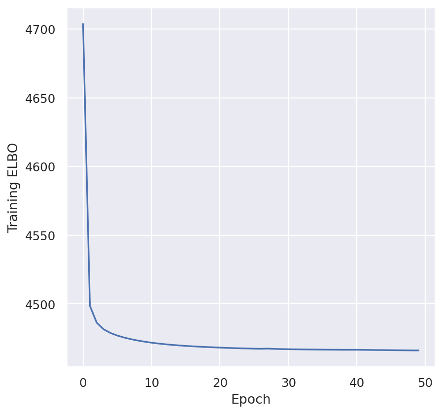
plt.plot(model.history["elbo_train"])
plt.xlabel("Epoch")
plt.ylabel("Training ELBO")
plt.show()

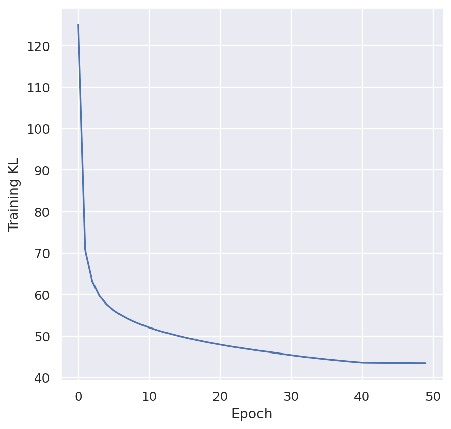
plt.plot(model.history["kl_local_train"])
plt.xlabel("Epoch")
plt.ylabel("Training KL")
plt.show()

# Save the model
model.save(
    "mrvi_torch_tahoe100_lamin_model", save_anndata=False, overwrite=True, datamodule=datamodule
)

# Load the model
# model = MRVI.load("mrvi_torch_tahoe100_lamin_model", adata=False)

# We extract the adata of the model, to be able to use it for plot umaps
# To save time we could also select a sub set of it
adata = collection.load(join="inner")
adata

AnnData object with n_obs × n_vars = 5000000 × 62710
    obs: 'drug', 'sample', 'BARCODE_SUB_LIB_ID', 'cell_line_id', 'moa-fine', 'canonical_smiles', 'pubchem_cid', 'plate', 'mean_gene_count', 'mean_tscp_count', 'mean_mread_count', 'mean_pcnt_mito', 'drugname_drugconc', 'targets', 'moa-broad', 'human-approved', 'clinical-trials', 'gpt-notes-approval', 'artifact_uid'

adata.obs.plate.value_counts()

plate
plate4     1141125
plate2     1084672
plate3     1056448
plate1     1028224
plate5      125045
plate10     112896
plate12     112896
plate11      84672
plate9       56450
plate7       56450
plate14      56448
plate6       28225
plate8       28225
plate13      28224
Name: count, dtype: int64

# merge metadata (will add memory)
# adata.obs = adata.obs.merge(tahoe_hubmodel.model.adata.obs[["Cell_Name_Vevo",
# "dataset","phase","observed_lib_size","S_score","G2M_score","sublibrary"]],
# how='left', left_on='BARCODE_SUB_LIB_ID', right_index=True)

adata

AnnData object with n_obs × n_vars = 5000000 × 62710
    obs: 'drug', 'sample', 'BARCODE_SUB_LIB_ID', 'cell_line_id', 'moa-fine', 'canonical_smiles', 'pubchem_cid', 'plate', 'mean_gene_count', 'mean_tscp_count', 'mean_mread_count', 'mean_pcnt_mito', 'drugname_drugconc', 'targets', 'moa-broad', 'human-approved', 'clinical-trials', 'gpt-notes-approval', 'artifact_uid'

# In order to save memory for the sake of this tutorial we drop the
# count matrix from this adata (like done during minification)
from scipy.sparse import csr_matrix

del adata.raw
adata.X = csr_matrix(adata.X.shape)

# The way to extract the internal model analysis is by the inference_dataloader
# Datamodule will always require to pass it into all downstream functions.
inference_dataloader = datamodule.inference_dataloader(
    batch_size=1024, parallel_cpu_count=5, shuffle=False
)

gc.collect()

9430

latent_representation = model.get_latent_representation(
    give_z=False, dataloader=inference_dataloader
)

latent_representation.shape

(5000000, 10)

We removed the count layer from the adata therefore we cant run PCA like before

# adata.layers["counts"] = adata.X.copy()  # preserve counts
# sc.pp.normalize_total(adata, target_sum=1e4)
# sc.pp.log1p(adata)
# adata.raw = adata  # freeze the state in `.raw`

# run PCA then generate UMAP plots
# sc.tl.pca(adata)
# sc.pp.neighbors(adata)
# sc.tl.umap(adata, min_dist=0.1)

# sc.pl.umap(
#    adata,
#    color=["plate", "cell_line_id"],
#    ncols=2,
#    frameon=False,
# )

adata.obsm["X_mrVI_Torch_Lamin"] = latent_representation

# Subsample the adata to save time and memory
adata_subsampled = adata[
    list(np.random.choice(np.arange(adata.n_obs), size=100000, replace=False)), :
].copy()

adata_subsampled.obsm["X_mrVI_Torch_Lamin"].shape

(100000, 10)

sc.pp.neighbors(adata_subsampled, use_rep="X_mrVI_Torch_Lamin")
sc.tl.umap(adata_subsampled, min_dist=0.3)

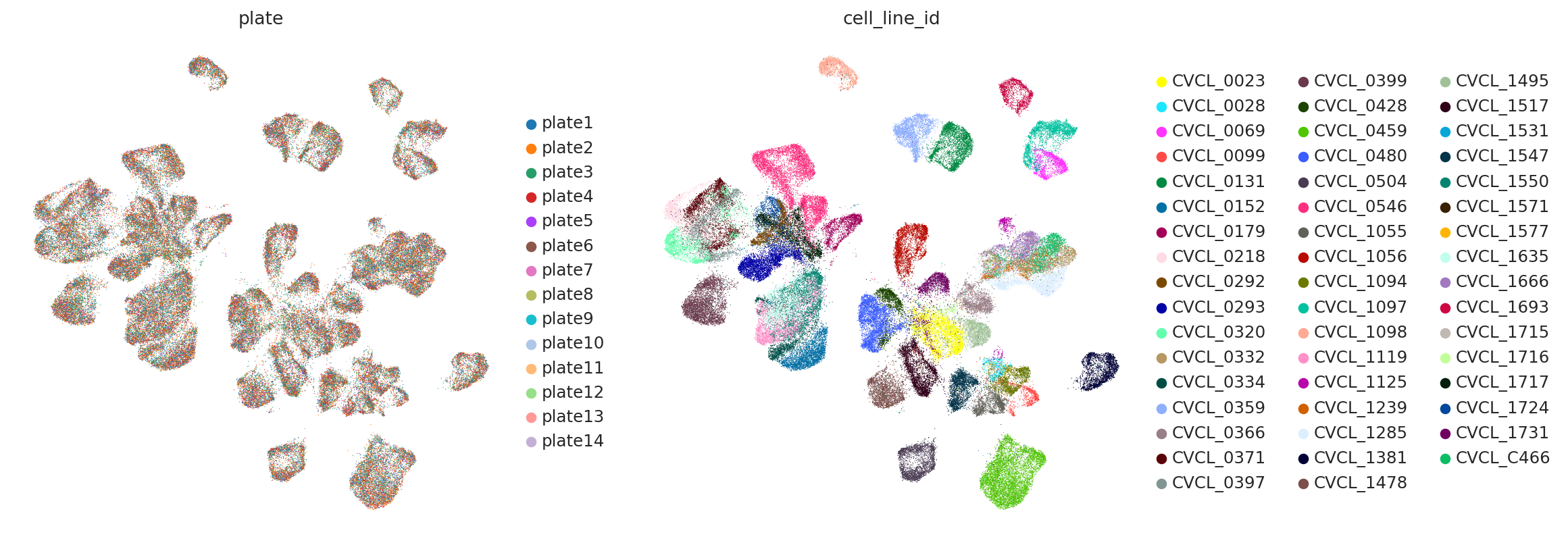
sc.pl.umap(
    adata_subsampled,
    color=["plate", "cell_line_id"],
    frameon=False,
    ncols=2,
)

We also didnt use the metadata

# sc.pl.umap(
#    adata,
#    color=["moa-broad","phase"],
#    frameon=False,
#    ncols=2,
# )

# sc.pl.umap(
#    adata,
#    color=["observed_lib_size","S_score","G2M_score"],
#    frameon=False,
#    ncols=3,
# )

Compare results

from scib_metrics.benchmark import BatchCorrection, Benchmarker, BioConservation

bm = Benchmarker(
    adata[list(np.random.choice(np.arange(adata.n_obs), size=10000, replace=False)), :],
    batch_key="plate",
    bio_conservation_metrics=BioConservation(
        isolated_labels=True,
        nmi_ari_cluster_labels_leiden=True,
        silhouette_label=True,
        clisi_knn=True,
        nmi_ari_cluster_labels_kmeans=True,
    ),
    batch_correction_metrics=BatchCorrection(
        bras=True,
        pcr_comparison=True,
        kbet_per_label=True,
        graph_connectivity=False,
        ilisi_knn=True,
    ),
    label_key="cell_line_id",
    embedding_obsm_keys=["X_mrVI_Torch_Lamin"],
    n_jobs=-1,
)
bm.benchmark()

bm.plot_results_table(min_max_scale=False)