ScBasset: Analyzing scATACseq data

Warning

SCBASSET’s development is still in progress. The current version may not fully reproduce the original implementation’s results.

Note

Running the following cell will install tutorial dependencies on Google Colab only. It will have no effect on environments other than Google Colab.

!pip install --quiet scvi-colab
from scvi_colab import install

install()

import tempfile

import matplotlib.pyplot as plt
import muon
import numpy as np
import scanpy as sc
import scvi
import seaborn as sns
import torch

scvi.settings.seed = 0
print("Last run with scvi-tools version:", scvi.__version__)

Note

You can modify save_dir below to change where the data files for this tutorial are saved.

sc.set_figure_params(figsize=(6, 6), frameon=False)
sns.set_theme()
torch.set_float32_matmul_precision("high")
save_dir = tempfile.TemporaryDirectory()

%config InlineBackend.print_figure_kwargs={"facecolor": "w"}
%config InlineBackend.figure_format="retina"

Loading data and preprocessing

Throughout this tutorial, we use sample multiome data from 10X of 10K PBMCs.

url = "https://cf.10xgenomics.com/samples/cell-arc/2.0.0/10k_PBMC_Multiome_nextgem_Chromium_X/10k_PBMC_Multiome_nextgem_Chromium_X_filtered_feature_bc_matrix.h5"
mdata = muon.read_10x_h5("data/multiome10k.h5mu", backup_url=url)

Added `interval` annotation for features from data/multiome10k.h5mu

mdata

MuData object with n_obs × n_vars = 10970 × 148344
  var:	'gene_ids', 'feature_types', 'genome', 'interval'
  2 modalities
    rna:	10970 x 36601
      var:	'gene_ids', 'feature_types', 'genome', 'interval'
    atac:	10970 x 111743
      var:	'gene_ids', 'feature_types', 'genome', 'interval'

adata = mdata.mod["atac"]

We can use scanpy functions to handle, filter, and manipulate the data. In our case, we might want to filter out peaks that are rarely detected, to make the model train faster:

print(adata.shape)
# compute the threshold: 5% of the cells
min_cells = int(adata.shape[0] * 0.05)
# in-place filtering of regions
sc.pp.filter_genes(adata, min_cells=min_cells)
print(adata.shape)

(10970, 111743)
(10970, 37054)

adata.var

	gene_ids	feature_types	genome	interval	n_cells
chr1:629395-630394	chr1:629395-630394	Peaks	GRCh38	chr1:629395-630394	1422
chr1:633578-634591	chr1:633578-634591	Peaks	GRCh38	chr1:633578-634591	4536
chr1:778283-779200	chr1:778283-779200	Peaks	GRCh38	chr1:778283-779200	5981
chr1:816873-817775	chr1:816873-817775	Peaks	GRCh38	chr1:816873-817775	564
chr1:827067-827949	chr1:827067-827949	Peaks	GRCh38	chr1:827067-827949	3150
...	...	...	...	...	...
GL000219.1:44739-45583	GL000219.1:44739-45583	Peaks	GRCh38	GL000219.1:44739-45583	781
GL000219.1:45726-46446	GL000219.1:45726-46446	Peaks	GRCh38	GL000219.1:45726-46446	639
GL000219.1:99267-100169	GL000219.1:99267-100169	Peaks	GRCh38	GL000219.1:99267-100169	6830
KI270726.1:41483-42332	KI270726.1:41483-42332	Peaks	GRCh38	KI270726.1:41483-42332	605
KI270713.1:21453-22374	KI270713.1:21453-22374	Peaks	GRCh38	KI270713.1:21453-22374	6247

37054 rows × 5 columns

split_interval = adata.var["gene_ids"].str.split(":", expand=True)
adata.var["chr"] = split_interval[0]
split_start_end = split_interval[1].str.split("-", expand=True)
adata.var["start"] = split_start_end[0].astype(int)
adata.var["end"] = split_start_end[1].astype(int)
adata.var

	gene_ids	feature_types	genome	interval	n_cells	chr	start	end
chr1:629395-630394	chr1:629395-630394	Peaks	GRCh38	chr1:629395-630394	1422	chr1	629395	630394
chr1:633578-634591	chr1:633578-634591	Peaks	GRCh38	chr1:633578-634591	4536	chr1	633578	634591
chr1:778283-779200	chr1:778283-779200	Peaks	GRCh38	chr1:778283-779200	5981	chr1	778283	779200
chr1:816873-817775	chr1:816873-817775	Peaks	GRCh38	chr1:816873-817775	564	chr1	816873	817775
chr1:827067-827949	chr1:827067-827949	Peaks	GRCh38	chr1:827067-827949	3150	chr1	827067	827949
...	...	...	...	...	...	...	...	...
GL000219.1:44739-45583	GL000219.1:44739-45583	Peaks	GRCh38	GL000219.1:44739-45583	781	GL000219.1	44739	45583
GL000219.1:45726-46446	GL000219.1:45726-46446	Peaks	GRCh38	GL000219.1:45726-46446	639	GL000219.1	45726	46446
GL000219.1:99267-100169	GL000219.1:99267-100169	Peaks	GRCh38	GL000219.1:99267-100169	6830	GL000219.1	99267	100169
KI270726.1:41483-42332	KI270726.1:41483-42332	Peaks	GRCh38	KI270726.1:41483-42332	605	KI270726.1	41483	42332
KI270713.1:21453-22374	KI270713.1:21453-22374	Peaks	GRCh38	KI270713.1:21453-22374	6247	KI270713.1	21453	22374

37054 rows × 8 columns

# Filter out non-chromosomal regions
mask = adata.var["chr"].str.startswith("chr")
adata = adata[:, mask].copy()

scvi.data.add_dna_sequence(
    adata,
    genome_name="GRCh38",
    genome_dir="data",
    chr_var_key="chr",
    start_var_key="start",
    end_var_key="end",
)
adata

Working...: 100%|██████████| 24/24 [00:02<00:00, 10.90it/s]

AnnData object with n_obs × n_vars = 10970 × 37042
    var: 'gene_ids', 'feature_types', 'genome', 'interval', 'n_cells', 'chr', 'start', 'end'
    varm: 'dna_sequence', 'dna_code'

adata.varm["dna_sequence"]

	0	1	2	3	4	5	6	7	8	9	...	1334	1335	1336	1337	1338	1339	1340	1341	1342	1343
chr1:629395-630394	C	A	C	T	C	T	C	C	C	C	...	C	T	A	T	A	T	C	T	A	A
chr1:633578-634591	G	A	A	A	T	A	G	G	G	C	...	T	A	A	A	T	C	C	C	C	T
chr1:778283-779200	C	G	C	C	C	G	G	C	T	A	...	G	A	C	A	G	G	A	G	T	T
chr1:816873-817775	A	A	T	T	C	A	T	A	T	G	...	T	T	A	G	C	G	G	C	T	G
chr1:827067-827949	C	T	C	T	C	C	T	G	C	C	...	C	G	T	T	A	T	T	A	A	T
...	...	...	...	...	...	...	...	...	...	...	...	...	...	...	...	...	...	...	...	...	...
chrY:19077075-19078016	A	C	G	A	C	C	T	C	C	C	...	C	A	T	A	G	T	T	C	T	A
chrY:19567013-19567787	G	G	A	G	T	C	T	G	G	G	...	T	C	T	C	T	T	C	G	T	T
chrY:19744368-19745303	T	A	T	T	T	T	T	G	T	C	...	A	T	G	T	G	G	A	A	A	T
chrY:20575244-20576162	T	T	T	A	C	T	G	T	C	T	...	G	A	G	T	G	T	A	A	C	A
chrY:21240021-21240909	A	T	T	G	G	C	C	C	C	C	...	C	C	T	T	T	C	T	G	A	G

37042 rows × 1344 columns

Creating and training the model

We can now set up the AnnData object, which will ensure everything the model needs is in place for training.

This is also the stage where we can condition the model on additional covariates, which encourages the model to remove the impact of those covariates from the learned latent space. Our sample data is a single batch, so we won’t demonstrate this directly, but it can be done simply by setting the batch_key argument to the annotation to be used as a batch covariate (must be a valid key in adata.obs) .

bdata = adata.transpose()
bdata.layers["binary"] = (bdata.X.copy() > 0).astype(float)
scvi.external.SCBASSET.setup_anndata(bdata, layer="binary", dna_code_key="dna_code")

INFO     Using column names from columns of adata.obsm['dna_code']                                                 

We can now create a scBasset model object and train it!

Note

The default max epochs is set to 1000, but in practice scBasset stops early once the model converges, which especially for large datasets (which require fewer epochs to converge, since each epoch includes letting the model view more data).

Here we are using 16 bit precision which uses less memory without sacrificing performance.

bas = scvi.external.SCBASSET(bdata)
bas.train(precision=16)

Epoch 724/1000:  72%|███████▏  | 724/1000 [1:18:18<29:51,  6.49s/it, v_num=1, train_loss_step=0.399, train_loss_epoch=0.362]
Monitored metric auroc_train did not improve in the last 45 records. Best score: 0.846. Signaling Trainer to stop.

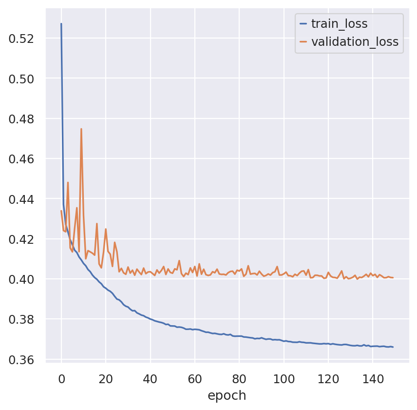
fig, ax = plt.subplots()
bas.history_["train_loss_epoch"].plot(ax=ax)
bas.history_["validation_loss"].plot(ax=ax)

<Axes: xlabel='epoch'>

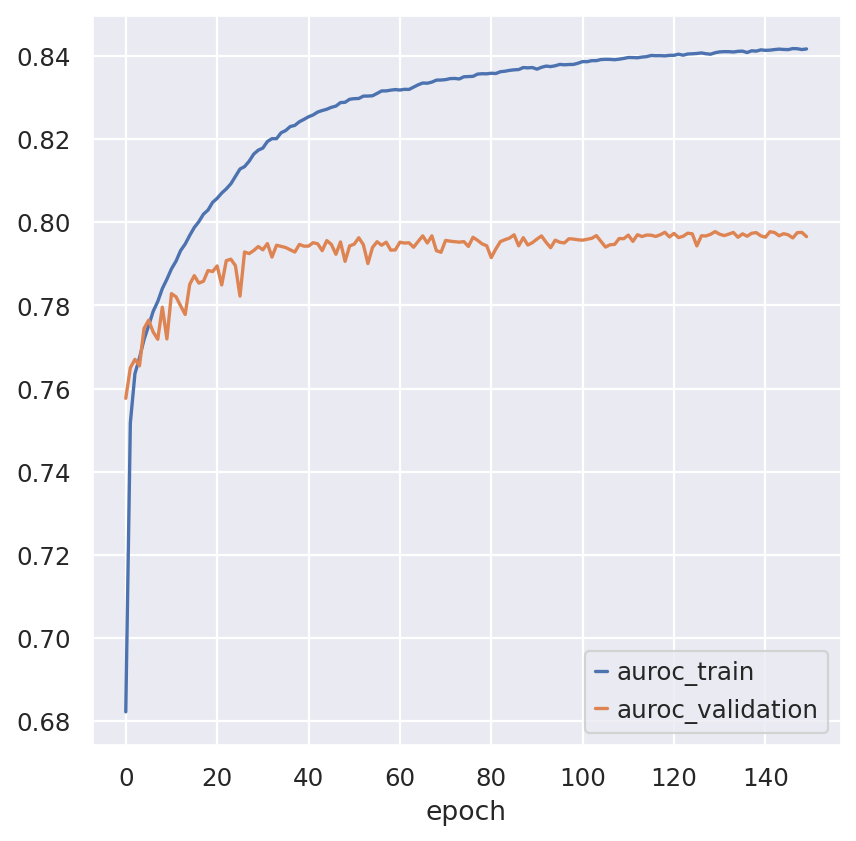
fig, ax = plt.subplots()
bas.history_["auroc_train"].plot(ax=ax)
bas.history_["auroc_validation"].plot(ax=ax)

<Axes: xlabel='epoch'>

Visualizing and analyzing the latent space

We can now use the trained model to visualize, cluster, and analyze the data. We first extract the latent representation from the model, and save it back into our AnnData object:

latent = bas.get_latent_representation()
adata.obsm["X_scbasset"] = latent

print(latent.shape)

(10970, 32)

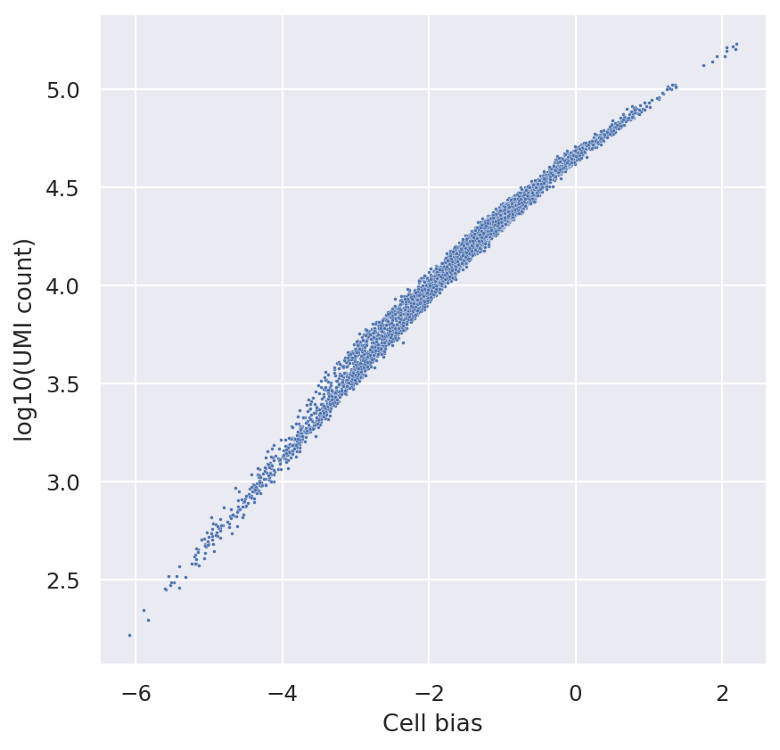
sns.scatterplot(
    x=bas.get_cell_bias(),
    y=np.log10(np.asarray(adata.X.sum(1))).ravel(),
    s=3,
)
plt.xlabel("Cell bias")
plt.ylabel("log10(UMI count)")

Text(0, 0.5, 'log10(UMI count)')

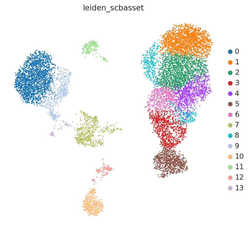
We can now use scanpy functions to cluster and visualize our latent space:

# compute the k-nearest-neighbor graph that is used in both clustering and umap algorithms
sc.pp.neighbors(adata, use_rep="X_scbasset")
# compute the umap
sc.tl.umap(adata)
sc.tl.leiden(adata, key_added="leiden_scbasset")

sc.pl.umap(adata, color="leiden_scbasset")

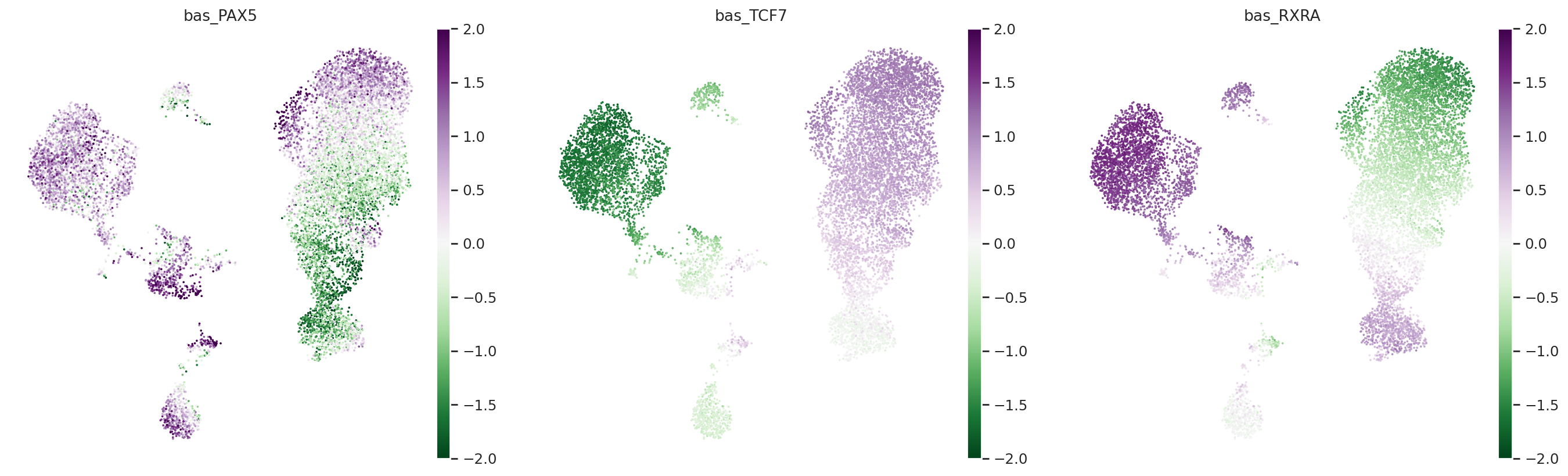
Score TF activity

We will now use the motif injection procedure to infer the activity of human transcription factors using their motifs.

This process involves downloading a library of (1) random dinucleotide shuffled sequences and (2) random sequences with a known motif injected. We infer the accessibility of all the random sequences and all the motif injected sequences in every cell using the SCBASSET model. We then compute the difference in activity for the motif injected sequences and the random sequences. This difference serves as an estimate for the likelihood that a given motif is accessible in each cell, and therefore an estimate of a corresponding transcription factor’s activity.

Any library with sequences of the appropriate size can be used. By default, we provide the human TF motif library used in the scBasset paper. The library is downloaded to a local folder (default: ./scbasset_motifs). Each motif is stored in a specific FASTA file in the {library_path}/shuffled_peaks_motifs subdirectory. To see all available motifs, simply glob the path (e.g. Path("./scbasset_motifs/shuffled_peaks_motifs").glob("*.fasta")).

tfs = ["PAX5", "TCF7", "RXRA"]

for tf in tfs:
    adata.obs[f"bas_{tf}"] = bas.get_tf_activity(
        tf=tf,
        motif_dir="data/motifs",
    )

INFO     Downloading motif set to: data/motifs                                                                     
INFO     Downloading file at data/motifs/human_motifs.tar.gz                                                       
Downloading...: 100%|██████████| 306466/306466.0 [00:06<00:00, 45712.42it/s]
INFO     Download and extraction complete.                                                                         

sc.pl.umap(
    adata,
    color=[f"bas_{tf}" for tf in tfs],
    cmap="PRGn_r",
    vmin=-2,
    vmax=2,
)