Integrating datasets with scVI in R#
In this tutorial, we go over how to use basic scvi-tools functionality in R. However, for more involved analyses, we suggest using scvi-tools from Python. Checkout the Scanpy_in_R tutorial for instructions on converting Seurat objects to anndata.
This tutorial requires Reticulate. Please check out our installation guide for instructions on installing Reticulate and scvi-tools.
Loading and processing data with Seurat#
We follow the basic Seurat tutorial for loading data and selecting highly variable genes.
Note: scvi-tools requires raw gene expression
# install.packages("Seurat")
# install.packages("reticulate")
# install.packages("cowplot")
# install.packages("devtools")

# devtools::install_github("satijalab/seurat-data")
# SeuratData::InstallData("pbmc3k")
# install.packages("https://seurat.nygenome.org/src/contrib/ifnb.SeuratData_3.0.0.tar.gz", repos = NULL, type = "source")
# SeuratData::InstallData("ifnb")

# devtools::install_github("cellgeni/sceasy")
# We will work within the Seurat framework
library(Seurat)
library(SeuratData)
data("pbmc3k")
pbmc <- pbmc3k

pbmc <- NormalizeData(pbmc, normalization.method = "LogNormalize", scale.factor = 10000)
pbmc[["percent.mt"]] <- PercentageFeatureSet(pbmc, pattern = "^MT-")
pbmc <- subset(pbmc, subset = nFeature_RNA > 200 & nFeature_RNA < 2500 & percent.mt < 5)
pbmc <- FindVariableFeatures(pbmc, selection.method = "vst", nfeatures = 2000)
top2000 <- head(VariableFeatures(pbmc), 2000)
pbmc <- pbmc[top2000]


print(pbmc) # Seurat object
An object of class Seurat
2000 features across 2638 samples within 1 assay
Active assay: RNA (2000 features, 2000 variable features)
Converting Seurat object to AnnData#
scvi-tools relies on the AnnData object. Here we show how to convert our Seurat object to anndata for scvi-tools.
library(reticulate)
library(sceasy)

sc <- import("scanpy", convert = FALSE)
scvi <- import("scvi", convert = FALSE)
adata <- convertFormat(pbmc, from="seurat", to="anndata", main_layer="counts", drop_single_values=FALSE)
print(adata) # Note generally in Python, dataset conventions are obs x var
AnnData object with n_obs × n_vars = 2638 × 2000
    obs: 'orig.ident', 'nCount_RNA', 'nFeature_RNA', 'seurat_annotations', 'percent.mt'
    var: 'vst.mean', 'vst.variance', 'vst.variance.expected', 'vst.variance.standardized', 'vst.variable'
Setup our AnnData for training#
Reticulate allows us to call Python code from R, giving the ability to use all of scvi-tools in R. We encourage you to checkout their documentation and specifically the section on type conversions in order to pass arguments to Python functions.
In this section, we show how to setup the AnnData for scvi-tools, create the model, train the model, and get the latent representation. For a more in depth description of setting up the data, you can checkout our introductory tutorial as well as our data loading tutorial.
# run setup_anndata
scvi$model$SCVI$setup_anndata(adata)

# create the model
model = scvi$model$SCVI(adata)

# train the model
model$train()

# to specify the number of epochs when training:
# model$train(max_epochs = as.integer(400))
None
None
Getting the latent represenation and visualization#
Here we get the latent representation of the model and save it back in our Seurat object. Then we run UMAP and visualize.
# get the latent represenation
latent = model$get_latent_representation()

# put it back in our original Seurat object
latent <- as.matrix(latent)
rownames(latent) = colnames(pbmc)
pbmc[["scvi"]] <- CreateDimReducObject(embeddings = latent, key = "scvi_", assay = DefaultAssay(pbmc))
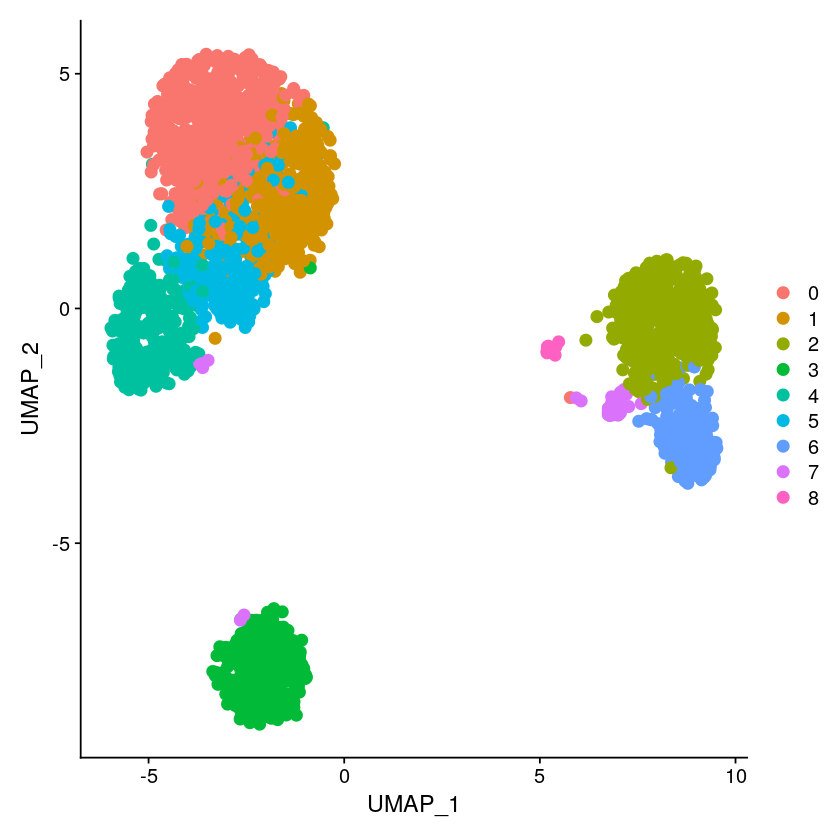
# Find clusters, then run UMAP, and visualize
pbmc <- FindNeighbors(pbmc, dims = 1:10, reduction = "scvi")
pbmc <- FindClusters(pbmc, resolution =1)

pbmc <- RunUMAP(pbmc, dims = 1:10, reduction = "scvi", n.components = 2)

DimPlot(pbmc, reduction = "umap", pt.size = 3)
Modularity Optimizer version 1.3.0 by Ludo Waltman and Nees Jan van Eck

Number of nodes: 2638
Number of edges: 91574

Running Louvain algorithm...
Maximum modularity in 10 random starts: 0.7180
Number of communities: 9
Elapsed time: 0 seconds
Finding differentially expressed genes with scVI latent space#
First, we put the seurat clusters into our original anndata.
adata$obs$insert(adata$obs$shape[1], "seurat_clusters", pbmc[["seurat_clusters"]][,1])
None
Using our trained SCVI model, we call the differential_expression() method
We pass seurat_clusters to the groupby argument and compare between cluster 1 and cluster 2.
The output of DE is a DataFrame with the bayes factors. Bayes factors > 3 have high probability of being differentially expressed. You can also set fdr_target, which will return the differentially expressed genes based on the posteior expected FDR.
DE <- model$differential_expression(adata, groupby="seurat_clusters", group1 = "1", group2 = "2")
print(DE$head())
        proba_de  proba_not_de  bayes_factor        scale1    scale2  ...  raw_normalized_mean2  is_de_fdr_0.05  comparison  group1  group2
S100A9    1.0000        0.0000     18.420681  4.506278e-04  0.032313  ...            402.134918            True      1 vs 2       1       2
LTB       1.0000        0.0000     18.420681  1.823797e-02  0.000625  ...              4.501131            True      1 vs 2       1       2
TNNT1     0.9998        0.0002      8.516943  5.922994e-07  0.000195  ...              0.781376            True      1 vs 2       1       2
TYMP      0.9998        0.0002      8.516943  4.944333e-04  0.004283  ...             46.068295            True      1 vs 2       1       2
IL7R      0.9998        0.0002      8.516943  4.791361e-03  0.000243  ...              1.657865            True      1 vs 2       1       2

[5 rows x 22 columns]
Integrating datasets with scVI#
Here we integrate two datasets from Seurat’s Immune Alignment Vignette.
data("ifnb")

# use seurat for variable gene selection
ifnb <- NormalizeData(ifnb, normalization.method = "LogNormalize", scale.factor = 10000)
ifnb[["percent.mt"]] <- PercentageFeatureSet(ifnb, pattern = "^MT-")
ifnb <- subset(ifnb, subset = nFeature_RNA > 200 & nFeature_RNA < 2500 & percent.mt < 5)
ifnb <- FindVariableFeatures(ifnb, selection.method = "vst", nfeatures = 2000)
top2000 <- head(VariableFeatures(ifnb), 2000)
ifnb <- ifnb[top2000]
adata <- convertFormat(ifnb, from="seurat", to="anndata", main_layer="counts", drop_single_values=FALSE)
print(adata)
AnnData object with n_obs × n_vars = 13997 × 2000
    obs: 'orig.ident', 'nCount_RNA', 'nFeature_RNA', 'stim', 'seurat_annotations', 'percent.mt'
    var: 'vst.mean', 'vst.variance', 'vst.variance.expected', 'vst.variance.standardized', 'vst.variable'
adata
AnnData object with n_obs × n_vars = 13997 × 2000
    obs: 'orig.ident', 'nCount_RNA', 'nFeature_RNA', 'stim', 'seurat_annotations', 'percent.mt'
    var: 'vst.mean', 'vst.variance', 'vst.variance.expected', 'vst.variance.standardized', 'vst.variable'
# run setup_anndata, use column stim for batch
scvi$model$SCVI$setup_anndata(adata, batch_key = 'stim')

# create the model
model = scvi$model$SCVI(adata)

# train the model
model$train()

# to specify the number of epochs when training:
# model$train(max_epochs = as.integer(400))
None
None
# get the latent represenation
latent = model$get_latent_representation()

# put it back in our original Seurat object
latent <- as.matrix(latent)
rownames(latent) = colnames(ifnb)
ifnb[["scvi"]] <- CreateDimReducObject(embeddings = latent, key = "scvi_", assay = DefaultAssay(ifnb))
library(cowplot)
# for jupyter notebook
options(repr.plot.width=10, repr.plot.height=8)
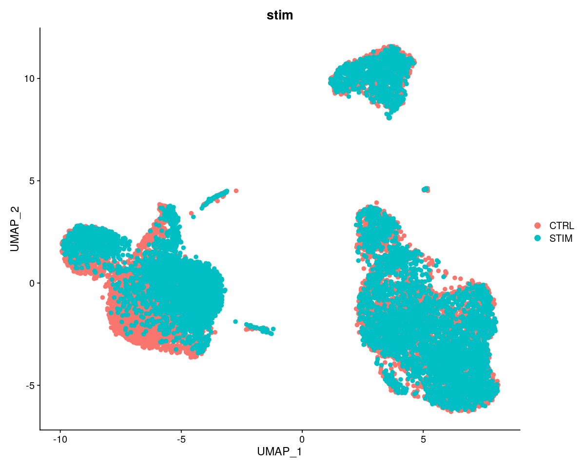
ifnb <- RunUMAP(ifnb, dims = 1:10, reduction = "scvi", n.components = 2)
p1 <- DimPlot(ifnb, reduction = "umap", group.by = "stim", pt.size=2)
plot_grid(p1)
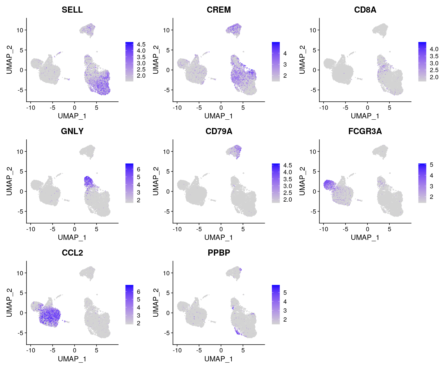
options(repr.plot.width=12, repr.plot.height=10)

FeaturePlot(ifnb, features = c("SELL", "CREM", "CD8A", "GNLY", "CD79A", "FCGR3A",
    "CCL2", "PPBP"), min.cutoff = "q9")
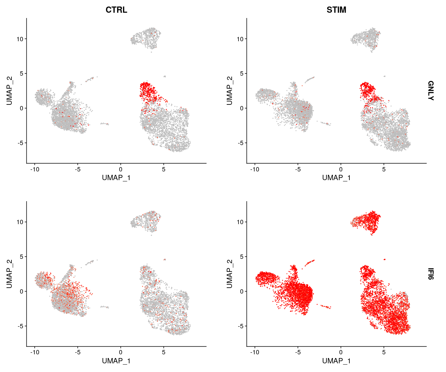
FeaturePlot(ifnb, features = c("GNLY", "IFI6"), split.by = "stim", max.cutoff = 3,
    cols = c("grey", "red"))
Session Info Summary#
sI <- sessionInfo()
sI$loadedOnly <- NULL
print(sI, locale=FALSE)
R version 4.0.3 (2020-10-10)
Platform: x86_64-conda-linux-gnu (64-bit)
Running under: Ubuntu 16.04.6 LTS

Matrix products: default
BLAS/LAPACK: /data/yosef2/users/jhong/miniconda3/envs/r_tutorial/lib/libopenblasp-r0.3.12.so

attached base packages:
[1] stats     graphics  grDevices utils     datasets  methods   base

other attached packages:
[1] cowplot_1.1.1             sceasy_0.0.6
[3] reticulate_1.22           stxBrain.SeuratData_0.1.1
[5] pbmc3k.SeuratData_3.1.4   ifnb.SeuratData_3.0.0
[7] SeuratData_0.2.1          SeuratObject_4.0.2
[9] Seurat_4.0.4