Multi-resolution deconvolution of spatial transcriptomics in R#
In this brief tutorial, we go over how to use scvi-tools functionality in R for analyzing spatial datasets. We will load spatial data following this Seurat tutorial, subsequently analyzing the data using DestVI.
This tutorial requires Reticulate. Please check out our installation guide for instructions on installing Reticulate and scvi-tools.
Loading and processing data with Seurat#
# install.packages("Seurat")
# install.packages("reticulate")
# install.packages("anndata")
# install.packages("devtools")
# devtools::install_github("satijalab/seurat-data")

# if (!requireNamespace("BiocManager", quietly = TRUE))
#     install.packages("BiocManager")

# BiocManager::install(c("LoomExperiment", "SingleCellExperiment"))
# devtools::install_github("cellgeni/sceasy")
library(Seurat)
library(SeuratData)
library(ggplot2)
First, we load the reference SMART-seq2 dataset of mouse brain. This dataset contains about 14,000 cells.
cortex_sc_data <- readRDS(url("https://www.dropbox.com/s/cuowvm4vrf65pvq/allen_cortex.rds?dl=1"))
InstallData("stxBrain")
brain_st_data <- LoadData("stxBrain", type = "anterior1")
Now, we subset the data in the same way that was done in the Seurat vignette, to match the cortex single-cell reference we are using.
brain_st_data <- SCTransform(brain_st_data, assay = "Spatial", verbose = FALSE)
brain_st_data <- RunPCA(brain_st_data, assay = "SCT", verbose = FALSE)
brain_st_data <- FindNeighbors(brain_st_data, reduction = "pca", dims = 1:30)
brain_st_data <- FindClusters(brain_st_data, verbose = FALSE)
brain_st_data <- RunUMAP(brain_st_data, reduction = "pca", dims = 1:30)

cortex_st_data <- subset(brain_st_data, idents = c(1, 2, 3, 4, 6, 7))
cortex_st_data <- subset(cortex_st_data, anterior1_imagerow > 400 | anterior1_imagecol < 150, invert = TRUE)
cortex_st_data <- subset(cortex_st_data, anterior1_imagerow > 275 & anterior1_imagecol > 370, invert = TRUE)
cortex_st_data <- subset(cortex_st_data, anterior1_imagerow > 250 & anterior1_imagecol > 440, invert = TRUE)
cortex_sc_data
An object of class Seurat
34617 features across 14249 samples within 1 assay
Active assay: RNA (34617 features, 0 variable features)
cortex_st_data
An object of class Seurat
48721 features across 1073 samples within 2 assays
Active assay: SCT (17668 features, 3000 variable features)
 1 other assay present: Spatial
 2 dimensional reductions calculated: pca, umap
cortex_sc_data <- NormalizeData(cortex_sc_data, normalization.method = "LogNormalize", scale.factor = 10000)
cortex_sc_data <- FindVariableFeatures(cortex_sc_data, selection.method = "vst", nfeatures = 2000)
top2000 <- head(VariableFeatures(cortex_sc_data), 2000)
top2000intersect <- intersect(rownames(cortex_st_data), top2000)
cortex_sc_data <- cortex_sc_data[top2000intersect]
cortex_st_data <- cortex_st_data[top2000intersect]
G <- length(top2000intersect)
G
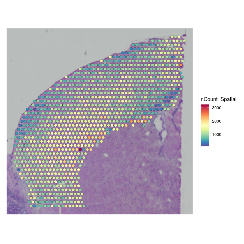
SpatialFeaturePlot(cortex_st_data, features = "nCount_Spatial") + theme(legend.position = "right")
Data conversion (Seurat -> AnnData)#
We use sceasy for conversion, and load the necessary Python packages for later.
library(reticulate)
library(sceasy)
library(anndata)

sc <- import("scanpy", convert = FALSE)
scvi <- import("scvi", convert = FALSE)
We make two AnnData objects, one for the single-cell reference and one for the spatial transcriptomics data, and then move the measurement coordinates to the appropriate attribute of the spatial AnnData.
cortex_sc_adata <- convertFormat(cortex_sc_data, from="seurat", to="anndata", main_layer="counts", drop_single_values=FALSE)
cortex_st_adata <- convertFormat(cortex_st_data, from="seurat", to="anndata", assay="Spatial", main_layer="counts", drop_single_values=FALSE)
Fit the scLVM#
scvi$model$CondSCVI$setup_anndata(cortex_sc_adata, labels_key="subclass")
None
Here we would like to reweight each measurement by a scalar factor (e.g., the inverse proportion) in the loss of the model so that lowly abundant cell types get better fit by the model.
sclvm <- scvi$model$CondSCVI(cortex_sc_adata, weight_obs=TRUE)
sclvm$train(max_epochs=as.integer(250))
None
# Make plot smaller.
saved <- options(repr.plot.width=6, repr.plot.height=5)
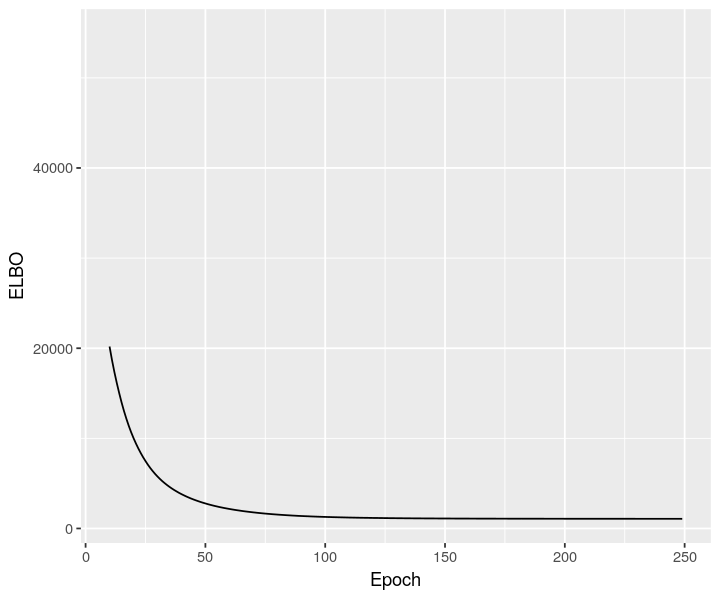
sclvm_elbo <- py_to_r(sclvm$history["elbo_train"]$astype("float64"))
ggplot(data = sclvm_elbo, mapping = aes(x=as.numeric(rownames(sclvm_elbo)), y=elbo_train)) + geom_line() + xlab("Epoch") + ylab("ELBO") + xlim(10, NA)
# Revert plot settings.
options(saved)
Deconvolution with stLVM#
scvi$model$DestVI$setup_anndata(cortex_st_adata)
None
stlvm <- scvi$model$DestVI$from_rna_model(cortex_st_adata, sclvm)
stlvm$train(max_epochs=as.integer(2500))
None
# Make plot smaller.
saved <- options(repr.plot.width=6, repr.plot.height=5)
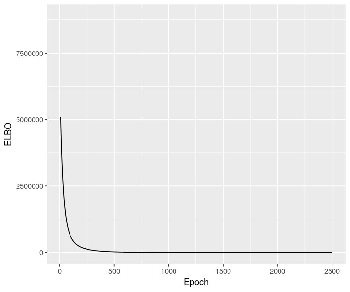
stlvm_elbo <- py_to_r(stlvm$history["elbo_train"]$astype("float64"))
ggplot(data = stlvm_elbo, mapping = aes(x=as.numeric(rownames(stlvm_elbo)), y=elbo_train)) + geom_line() + xlab("Epoch") + ylab("ELBO") + xlim(10, NA)
# Revert plot settings.
options(saved)
Cell type proportions#
cortex_st_adata$obsm["proportions"] <- stlvm$get_proportions()
head(py_to_r(cortex_st_adata$obsm$get("proportions")))
| Astro | CR | Endo | L2/3 IT | L4 | L5 IT | L5 PT | L6 CT | L6 IT | L6b | ⋯ | NP | Oligo | Peri | Pvalb | SMC | Serpinf1 | Sncg | Sst | VLMC | Vip | |
|---|---|---|---|---|---|---|---|---|---|---|---|---|---|---|---|---|---|---|---|---|---|
| <dbl> | <dbl> | <dbl> | <dbl> | <dbl> | <dbl> | <dbl> | <dbl> | <dbl> | <dbl> | ⋯ | <dbl> | <dbl> | <dbl> | <dbl> | <dbl> | <dbl> | <dbl> | <dbl> | <dbl> | <dbl> | |
| AAACAGAGCGACTCCT-1 | 0.132741362 | 0.008747282 | 0.011718361 | 0.221762791 | 0.0070496136 | 0.1546385437 | 0.077167749 | 0.0005695362 | 0.069925420 | 0.152741432 | ⋯ | 0.0007827459 | 0.010729197 | 0.023100458 | 0.0039191837 | 0.010946345 | 0.0147322891 | 0.0147522716 | 0.001043379 | 0.003957638 | 0.0138991615 |
| AAACCGGGTAGGTACC-1 | 0.184176832 | 0.003791695 | 0.005254562 | 0.234996960 | 0.0800886825 | 0.0067960601 | 0.048472349 | 0.0326679721 | 0.091120958 | 0.001587714 | ⋯ | 0.0635546148 | 0.001604313 | 0.002388439 | 0.0015827275 | 0.010713122 | 0.0008687067 | 0.0090936236 | 0.063255355 | 0.055150922 | 0.0461300276 |
| AAACCGTTCGTCCAGG-1 | 0.012769192 | 0.018516796 | 0.084555522 | 0.002121322 | 0.0692796335 | 0.0043616821 | 0.001594895 | 0.0711863041 | 0.003215992 | 0.009484144 | ⋯ | 0.0029538164 | 0.023589995 | 0.018594360 | 0.0465325005 | 0.199640453 | 0.0400414765 | 0.0009976953 | 0.051015414 | 0.267024368 | 0.0210210774 |
| AAACTCGTGATATAAG-1 | 0.001966703 | 0.001308091 | 0.003387878 | 0.001047674 | 0.0006783445 | 0.0022771859 | 0.001468480 | 0.1649082154 | 0.005263278 | 0.601306736 | ⋯ | 0.0017696184 | 0.176176697 | 0.001715337 | 0.0002066867 | 0.001542291 | 0.0004248595 | 0.0003984653 | 0.000195155 | 0.001623075 | 0.0003795118 |
| AAAGGGATGTAGCAAG-1 | 0.092700399 | 0.000697523 | 0.020046912 | 0.127878055 | 0.1897880286 | 0.1099940836 | 0.077412799 | 0.0014952135 | 0.006032379 | 0.001297700 | ⋯ | 0.0023012036 | 0.017050896 | 0.001693511 | 0.1491737664 | 0.018952442 | 0.0049221730 | 0.0014064765 | 0.112875126 | 0.014681718 | 0.0166219342 |
| AAATAACCATACGGGA-1 | 0.147560343 | 0.008129421 | 0.033958640 | 0.391459972 | 0.0033571674 | 0.0007401044 | 0.016744409 | 0.0909470767 | 0.146570548 | 0.004010124 | ⋯ | 0.0007179513 | 0.004490611 | 0.004775111 | 0.0008306661 | 0.001726551 | 0.0103975814 | 0.0006136570 | 0.001548895 | 0.005978103 | 0.0521079451 |
cortex_st_data[["predictions"]] <- CreateAssayObject(data = t(py_to_r(cortex_st_adata$obsm$get("proportions"))))
DefaultAssay(cortex_st_data) <- "predictions"
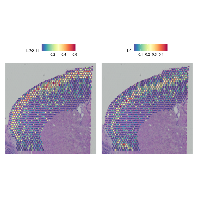
SpatialFeaturePlot(cortex_st_data, features = c("L2/3 IT", "L4"), pt.size.factor = 1.6, ncol = 2, crop = TRUE)
Intra cell type information#
At the heart of DestVI is a multitude of latent variables (5 per cell type per spots). We refer to them as “gamma”, and we may manually examine them for downstream analysis.
Because those values may be hard to examine for end-users, we presented several methods for prioritizing the study of different cell types (based on PCA and Hotspot). If you’d like to use those methods, please refer to our DestVI reproducibility repository. If you have suggestions to improve those, and would like to see them in the main codebase, reach out to us.
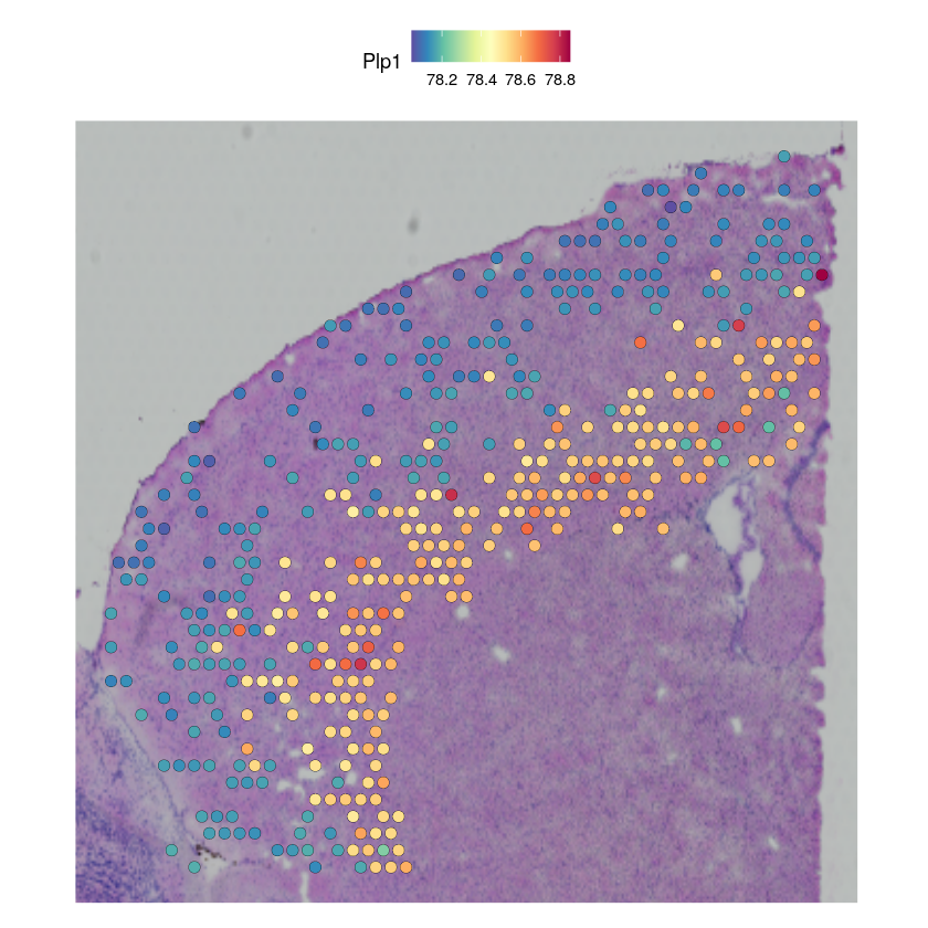
In this tutorial, we assume that the user have identified key gene modules that vary within one cell type in the single-cell RNA sequencing data (e.g., using Hotspot). We provide here a code snippet for imputing the spatial pattern of the cell type specific gene expression, using the example of the PLP1 gene in Endothelial cells.
for (cell_type_gamma in iterate(stlvm$get_gamma()$items())) {
    cell_type <- cell_type_gamma[0]
    gamma_df <- cell_type_gamma[1]
    cortex_st_data[[paste(cell_type, "_gamma", sep = "")]] <- CreateAssayObject(data = t(py_to_r(gamma_df)))
}
head(GetAssayData(cortex_st_data))
| AAACAGAGCGACTCCT-1 | AAACCGGGTAGGTACC-1 | AAACCGTTCGTCCAGG-1 | AAACTCGTGATATAAG-1 | AAAGGGATGTAGCAAG-1 | AAATAACCATACGGGA-1 | AAATCGTGTACCACAA-1 | AAATGATTCGATCAGC-1 | AAATGGTCAATGTGCC-1 | AAATTAACGGGTAGCT-1 | ⋯ | TTGGTCACACTCGTAA-1 | TTGTAAGGACCTAAGT-1 | TTGTAAGGCCAGTTGG-1 | TTGTAATCCGTACTCG-1 | TTGTCGTTCAGTTACC-1 | TTGTGGCCCTGACAGT-1 | TTGTGTTTCCCGAAAG-1 | TTGTTCAGTGTGCTAC-1 | TTGTTGTGTGTCAAGA-1 | TTGTTTCCATACAACT-1 | |
|---|---|---|---|---|---|---|---|---|---|---|---|---|---|---|---|---|---|---|---|---|---|
| Astro | 0.132741362 | 0.184176832 | 0.012769192 | 0.0019667035 | 0.092700399 | 0.1475603431 | 0.0004045009 | 0.031076301 | 0.136070669 | 0.0197930187 | ⋯ | 0.1365053356 | 0.08824219 | 0.087588087 | 0.081193000 | 0.1984594613 | 0.281091094 | 0.016215326 | 0.081116490 | 0.061543569 | 0.1241387874 |
| CR | 0.008747282 | 0.003791695 | 0.018516796 | 0.0013080909 | 0.000697523 | 0.0081294207 | 0.0063187955 | 0.003309071 | 0.003154238 | 0.0008858569 | ⋯ | 0.0037494451 | 0.03061977 | 0.003443674 | 0.001939139 | 0.0097711813 | 0.003028526 | 0.026655646 | 0.001710637 | 0.005380775 | 0.1895391792 |
| Endo | 0.011718361 | 0.005254562 | 0.084555522 | 0.0033878782 | 0.020046912 | 0.0339586399 | 0.0019674290 | 0.039658114 | 0.051655442 | 0.0185621772 | ⋯ | 0.0050291684 | 0.02816591 | 0.001338468 | 0.052013196 | 0.0486835353 | 0.026372865 | 0.012466145 | 0.043418083 | 0.046080951 | 0.0098529318 |
| L2/3 IT | 0.221762791 | 0.234996960 | 0.002121322 | 0.0010476735 | 0.127878055 | 0.3914599717 | 0.0094522228 | 0.001090960 | 0.052895129 | 0.0520999767 | ⋯ | 0.0052948804 | 0.16736636 | 0.003720999 | 0.004698100 | 0.1383295357 | 0.169778779 | 0.004306178 | 0.265172213 | 0.002287487 | 0.0017337656 |
| L4 | 0.007049614 | 0.080088682 | 0.069279633 | 0.0006783445 | 0.189788029 | 0.0033571674 | 0.0009997272 | 0.097140528 | 0.060398243 | 0.0105798170 | ⋯ | 0.0224371944 | 0.01600794 | 0.146402493 | 0.011464869 | 0.1294399202 | 0.123409927 | 0.016023967 | 0.003908478 | 0.001758869 | 0.0001608078 |
| L5 IT | 0.154638544 | 0.006796060 | 0.004361682 | 0.0022771859 | 0.109994084 | 0.0007401044 | 0.1498650759 | 0.039135456 | 0.385494292 | 0.1260202378 | ⋯ | 0.0008620349 | 0.00132572 | 0.206354573 | 0.103019625 | 0.0007694541 | 0.002617676 | 0.122893602 | 0.002557966 | 0.207107291 | 0.0006238798 |
ct_name <- "L6 IT"
gene_name <- "Plp1"

# filter for spots with low abundance
indices <- which(GetAssayData(cortex_st_data$predictions)[ct_name,] > 0.03)

# impute gene
specific_expression <- stlvm$get_scale_for_ct(ct_name, indices = r_to_py(as.integer(indices - 1)))[[gene_name]]
specific_expression <- 1 + 1e4 * py_to_r(specific_expression$to_frame())
filtered_st_data <- cortex_st_data[, indices]
filtered_st_data[["imputation"]] <- CreateAssayObject(data = t(specific_expression))
DefaultAssay(filtered_st_data) <- "imputation"
SpatialFeaturePlot(filtered_st_data, features = gene_name)
Session Info#
sI <- sessionInfo()
sI$loadedOnly <- NULL
print(sI, locale=FALSE)
R version 4.0.3 (2020-10-10)
Platform: x86_64-conda-linux-gnu (64-bit)
Running under: Ubuntu 16.04.6 LTS

Matrix products: default
BLAS/LAPACK: /data/yosef2/users/jhong/miniconda3/envs/r_tutorial/lib/libopenblasp-r0.3.12.so

attached base packages:
[1] stats     graphics  grDevices utils     datasets  methods   base

other attached packages:
 [1] anndata_0.7.5.3           sceasy_0.0.6
 [3] reticulate_1.22           ggplot2_3.3.5
 [5] stxBrain.SeuratData_0.1.1 pbmc3k.SeuratData_3.1.4
 [7] ifnb.SeuratData_3.0.0     SeuratData_0.2.1
 [9] SeuratObject_4.0.2        Seurat_4.0.4