Atlas-level integration of lung data#
An important task of single-cell analysis is the integration of several samples, which we can perform with scVI. For integration, scVI treats the data as unlabelled. When our dataset is fully labelled (perhaps in independent studies, or independent analysis pipelines), we can obtain an integration that better preserves biology using scANVI, which incorporates cell type annotation information. Here we demonstrate this functionality with an integrated analysis of cells from the lung atlas integration task from the scIB manuscript. The same pipeline would generally be used to analyze any collection of scRNA-seq datasets.
Note
Running the following cell will install tutorial dependencies on Google Colab only. It will have no effect on environments other than Google Colab.
!pip install --quiet scvi-colab
from scvi_colab import install

install()
import os
import tempfile

import scanpy as sc
import scvi
import seaborn as sns
import torch
from rich import print
from scib_metrics.benchmark import Benchmarker
scvi.settings.seed = 0
print("Last run with scvi-tools version:", scvi.__version__)
Last run with scvi-tools version: 1.4.2
Note
You can modify save_dir below to change where the data files for this tutorial are saved.
sc.set_figure_params(figsize=(6, 6), frameon=False)
sns.set_theme()
torch.set_float32_matmul_precision("high")
save_dir = tempfile.TemporaryDirectory()

%config InlineBackend.print_figure_kwargs={"facecolor": "w"}
%config InlineBackend.figure_format="retina"
Dataset Preprocessing#
For this tutorial we use an already preprocessed dataset from the lung atlas integration task in the scIB manuscript. To see the exact preprocessing that was done, or to preprocess your own scRNA dataset for use with scvi-tools models, see our preprocessing tutorial.
# download preprocessed dataset
adata_path = os.path.join(save_dir.name, "lung_atlas_preprocessed.h5ad")

adata = sc.read(
    adata_path,
    backup_url="https://exampledata.scverse.org/scvi-tools/lung_atlas_preprocessed.h5ad",
)
adata
AnnData object with n_obs × n_vars = 32472 × 2000
    obs: 'dataset', 'location', 'nGene', 'nUMI', 'patientGroup', 'percent.mito', 'protocol', 'sanger_type', 'size_factors', 'sampling_method', 'batch', 'cell_type', 'donor'
    var: 'highly_variable', 'highly_variable_rank', 'means', 'variances', 'variances_norm', 'highly_variable_nbatches'
    uns: 'hvg'
    layers: 'counts'
Integration with scVI#
As a first step, we assume that the data is completely unlabelled and we wish to find common axes of variation between the two datasets. There are many methods available in scanpy for this purpose (BBKNN, Scanorama, etc.). In this notebook we present scVI. To run scVI, we simply need to:
Register the AnnData object with the correct key to identify the sample and the layer key with the count data.
Create an SCVI model object.
scvi.model.SCVI.setup_anndata(adata, layer="counts", batch_key="batch")
We note that these parameters are non-default; however, they have been verified to generally work well in the integration task.
model = scvi.model.SCVI(adata, n_layers=2, n_latent=30, gene_likelihood="nb")
Now we train scVI. This should take a couple of minutes on a Colab session
model.train()
Once the training is done, we can evaluate the latent representation of each cell in the dataset and add it to the AnnData object
SCVI_LATENT_KEY = "X_scVI"
adata.obsm[SCVI_LATENT_KEY] = model.get_latent_representation()
Finally, we can cluster the dataset and visualize it the scVI latent space.
sc.pp.neighbors(adata, use_rep=SCVI_LATENT_KEY)
sc.tl.leiden(adata)
To visualize the scVI’s learned embeddings, we use UMAP.
sc.tl.umap(adata, min_dist=0.3)
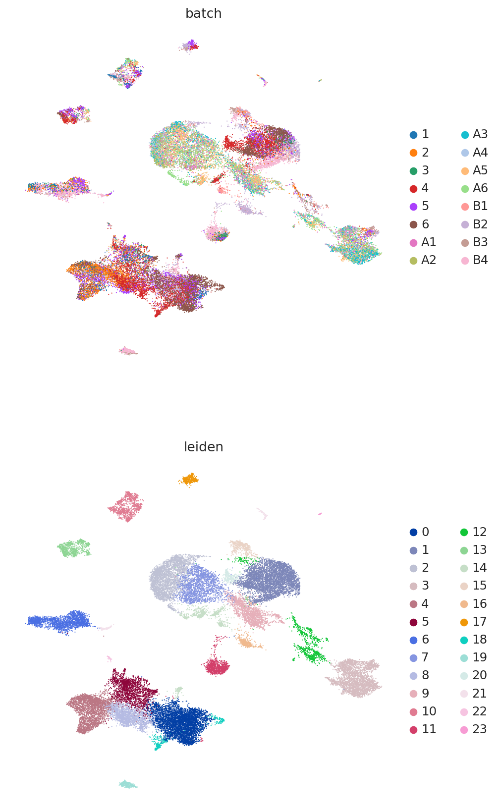
sc.pl.umap(
adata,
color=["batch", "leiden"],
frameon=False,
ncols=1,
)
Because this data has been used for benchmarking, we have access here to curated annotations. We can use those to assess whether the integration worked reasonably well.
sc.pl.umap(
    adata,
    color=["cell_type"],
    frameon=False,
    ncols=1,
)
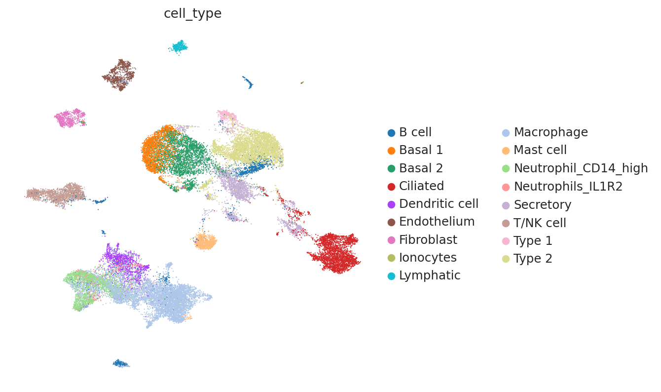
At a quick glance, it looks like the integration worked well. Indeed, the two datasets are relatively mixed in latent space and the cell types cluster together. We see that this dataset is quite complex, where only some batches contain certain cell types.
Below we quantify the performance.
Integration with scANVI#
Previously, we used scVI as we assumed we did not have any cell type annotations available to guide us. Consequently, after the previous analysis, one would have to annotate clusters using differential expression, or by other means.
Now, we assume that all of our data is annotated. This can lead to a more accurate integration result when using scANVI, i.e., our latent data manifold is better suited to downstream tasks like visualization, trajectory inference, or nearest-neighbor-based tasks. scANVI requires:
the sample identifier for each cell (as in scVI)
the cell type/state for each cell
scANVI can also be used for label transfer and we recommend checking out the other scANVI tutorials to see explore this functionality.
Since we’ve already trained an scVI model on our data, we will use it to initialize scANVI. When initializing scANVI, we provide it the labels_key. As scANVI can also be used for datasets with partially-observed annotations, we need to give it the name of the category that corresponds to unlabeled cells. As we have no unlabeled cells, we can give it any random name that is not the name of an exisiting cell type.
Important
scANVI should be initialized from a scVI model pre-trained on the same exact data.
scanvi_model = scvi.model.SCANVI.from_scvi_model(
    model,
    adata=adata,
    labels_key="cell_type",
    unlabeled_category="Unknown",
)
scanvi_model.train(max_epochs=20, n_samples_per_label=100)
INFO Training for 20 epochs.
Now we can retrieve the latent space
SCANVI_LATENT_KEY = "X_scANVI"
adata.obsm[SCANVI_LATENT_KEY] = scanvi_model.get_latent_representation(adata)
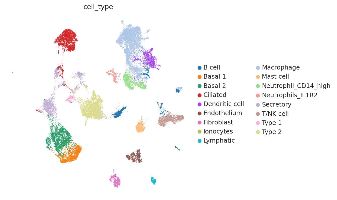
Again, we may visualize the latent space as well as the inferred labels
sc.pp.neighbors(adata, use_rep=SCANVI_LATENT_KEY)
sc.tl.umap(adata, min_dist=0.3)
sc.pl.umap(
    adata,
    color=["cell_type"],
    frameon=False,
    ncols=1,
)
Compute integration metrics#
Here we use the scib-metrics package, which contains scalable implementations of the metrics used in the scIB benchmarking suite. We can use these metrics to assess the quality of the integration.
We can see that the additional training with label information and scANVI improved the metrics that capture bio conservation (cLISI, Silhouette labels) without sacrificing too much batch correction power (iLISI, Silhouette batch)
bm = Benchmarker(
    adata,
    batch_key="batch",
    label_key="cell_type",
    embedding_obsm_keys=["X_pca", SCVI_LATENT_KEY, SCANVI_LATENT_KEY],
    n_jobs=-1,
)
bm.benchmark()
bm.plot_results_table(min_max_scale=False)
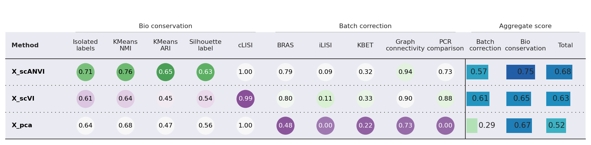
<plottable.table.Table at 0x7e51a048fa10>
df = bm.get_results(min_max_scale=False)
print(df)
              Isolated labels        KMeans NMI        KMeans ARI  \
Embedding
X_pca                 0.64364          0.676374          0.468682
X_scVI               0.611918           0.64014          0.446901
X_scANVI             0.705827          0.764504           0.65176
Metric Type  Bio conservation  Bio conservation  Bio conservation

             Silhouette label             cLISI              BRAS  \
Embedding
X_pca                0.557418               1.0          0.484245
X_scVI               0.537654          0.993558          0.803095
X_scANVI             0.625365               1.0          0.787167
Metric Type  Bio conservation  Bio conservation  Batch correction

                        iLISI              KBET Graph connectivity  \
Embedding
X_pca                0.003445          0.222977           0.728504
X_scVI               0.114577          0.332003           0.903552
X_scANVI             0.085612          0.318977           0.942232
Metric Type  Batch correction  Batch correction   Batch correction

               PCR comparison Batch correction Bio conservation  \
Embedding
X_pca                     0.0         0.287834         0.669223
X_scVI               0.881288         0.606903         0.646034
X_scANVI              0.72992         0.572782         0.749491
Metric Type  Batch correction  Aggregate score  Aggregate score

                       Total
Embedding
X_pca               0.516667
X_scVI              0.630382
X_scANVI            0.678807
Metric Type  Aggregate score