Decipher Quick Start Tutorial

Decipher is a model for jointly analyzing single-cell RNA-seq samples from distinct conditions (e.g. normal vs perturbed samples). This tutorial will guide you through the steps to use Decipher to analyze a dataset.

Note: This tutorial currently only features a basic Decipher model. A more fleshed out implemention aligned with the original implementation is currently in development and will be released soon along with updates to this tutorial.

!pip install --quiet scvi-colab
from scvi_colab import install

install()

import os
import tempfile

import matplotlib.pyplot as plt
import scanpy as sc
import scvi
from scvi.external import Decipher

scvi.settings.seed = 0  # optional: ensures reproducibility
print("Last run with scvi-tools version:", scvi.__version__)
save_dir = tempfile.TemporaryDirectory()

Last run with scvi-tools version: 1.3.0

Preprocessing and model fitting

For this tutorial, we will use a subset of the AML data from the Decipher preprint for the purpose of demonstrating how to use Decipher with scvi-tools.

adata_path = os.path.join(save_dir.name, "decipher_tutorial_data.h5ad")

adata = sc.read(
    adata_path,
    backup_url="https://github.com/azizilab/decipher_data/raw/refs/heads/main/data_decipher_tutorial.h5ad",
)
adata = adata[
    ~adata.obs["cell_type"].isin(["mep", "ery", "lympho"])
].copy()  # subset to only include relevant cell types

adata

AnnData object with n_obs × n_vars = 16627 × 3130
    obs: 'cell_type', 'origin', 'NPM1 mutation vs wild type'
    uns: 'color_palette', 'decipher'
    obsm: 'X_pca', 'X_tsne', 'decipher_v', 'decipher_z'
    varm: 'PCs'
    obsp: 'connectivities', 'distances'

Decipher does not require any additional covariates, and only optionally takes a layer indicating which layer of the AnnData object contains the raw count data.

Decipher.setup_anndata(adata)

Now we are ready to fit the model.

model = Decipher(adata)
model.train(
    max_epochs=100,
    batch_size=64,
    early_stopping=True,
    early_stopping_patience=10,
)

Monitored metric nll_validation did not improve in the last 10 records. Best score: 3489.798. Signaling Trainer to stop.

# save load functionality
save_path = f"./_decipher_models/test_notebook_model_{scvi.settings.seed}"
model.save(save_path, overwrite=True)
model = Decipher.load(save_path, adata)

INFO     File ./_decipher_models/test_notebook_model_0/model.pt already downloaded

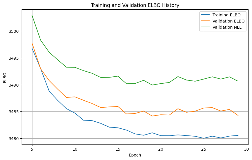
# Plot training and validation ELBO history
plt.figure(figsize=(10, 6))
plt.plot(model.history_["elbo_train"][5:], label="Training ELBO")
plt.plot(model.history_["elbo_validation"][5:], label="Validation ELBO")
plt.plot(model.history_["nll_validation"][5:], label="Validation NLL")
plt.xlabel("Epoch")
plt.ylabel("ELBO")
plt.title("Training and Validation ELBO History")
plt.legend()
plt.grid(True)
plt.show()

Visualize the latent representation

Now that we have confirmed the model has converged, we can visualize the latent representation.

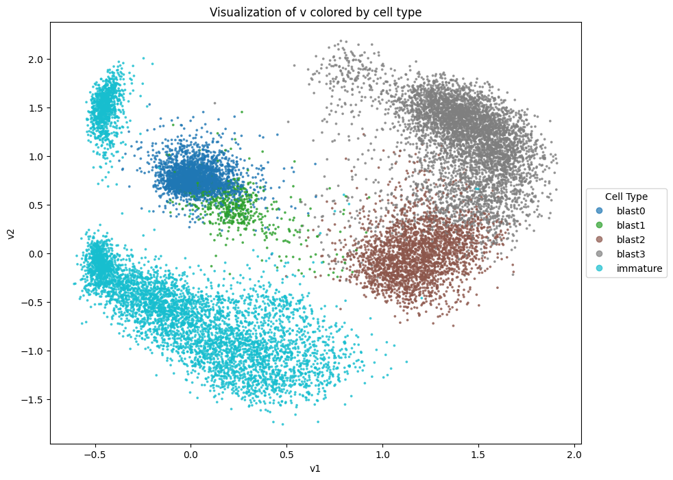
Notably, Decipher has two latent representations: v and z. v is a 2-dimensional latent representation which is amenable to direct visualization, while z is a higher-dimensional latent representation which is designed to capture more refined cell state information such as transitional intermediates.

v = model.get_latent_representation()
# Plot v and color by cell type
cell_type_mapping = adata.obs["cell_type"].astype("category").cat
plt.figure(figsize=(10, 8))
scatter = plt.scatter(v[:, 0], v[:, 1], c=cell_type_mapping.codes, cmap="tab10", alpha=0.7, s=3)

plt.legend(
    scatter.legend_elements()[0],
    cell_type_mapping.categories,
    title="Cell Type",
    loc="center left",
    bbox_to_anchor=(1, 0.5),
)

plt.title("Visualization of v colored by cell type")
plt.xlabel("v1")
plt.ylabel("v2")
plt.show()

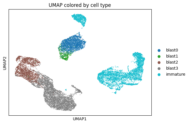
z = model.get_latent_representation(give_z=True)
adata.obsm["z"] = z
sc.pp.neighbors(adata, use_rep="z")
sc.tl.umap(adata, min_dist=0.3)
sc.pl.umap(
    adata,
    color=["cell_type"],
    frameon=True,
    palette="tab10",
    ncols=1,
    title="UMAP colored by cell type",
)